Resize

Overview

The resize module in SplineOps provides high-performance, high-fidelity resizing for N-dimensional arrays.

This module allows us to obtain classical standard cubic interpolation (see following animation, at left) and high-quality antialiasing projection-based (see following animation, at right).

This animation and its details are available in the example Resize Module 2D.

Conceptually, resizing means:

• starting from a spline \(f\) defined on an input grid (typically the integers),

• choosing a new output grid, obtained by scaling the grid by a factor \(T\) (e.g., \(0, T, 2T, 3T, \dots\)),

• and constructing a new spline \(g\) that “lives” on that new grid and best represents the same underlying continuous function.

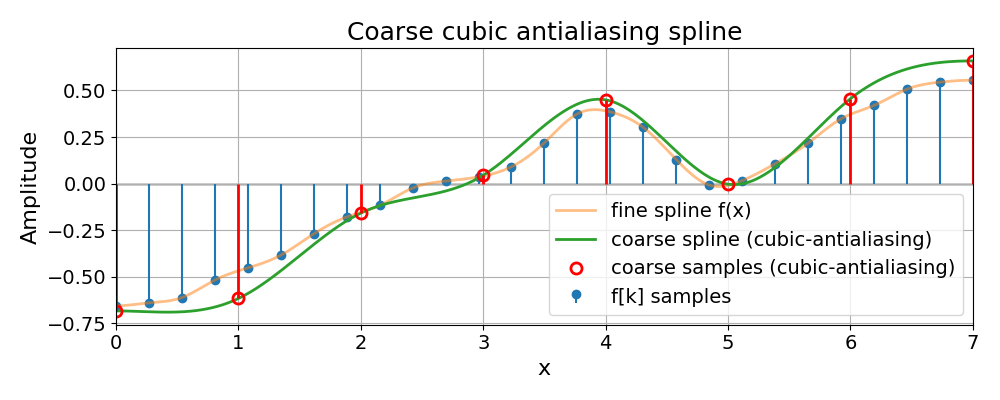
We illustrate this with the 1D example Resample a 1D Spline, which starts from a spline \(f\) and samples it more coarsely at positions \(x = T k\):

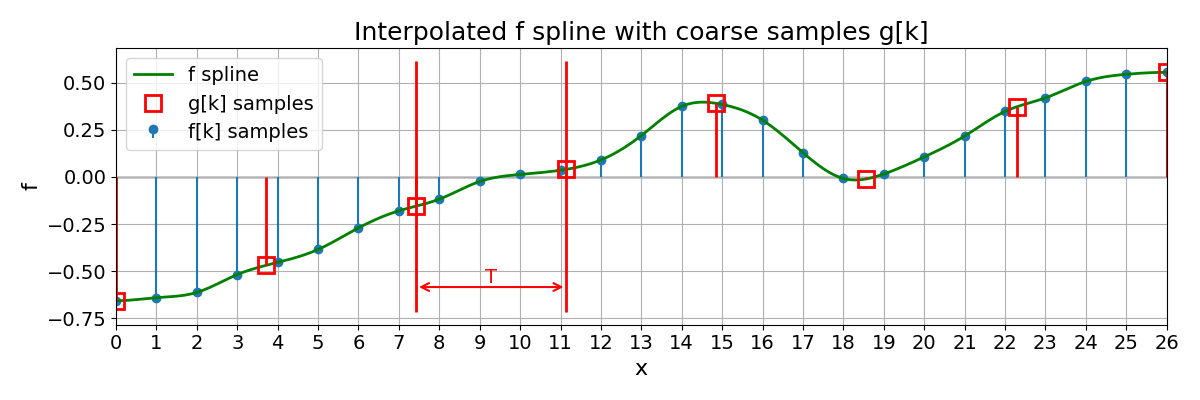
The red stems and markers correspond to the new samples \(f(Tk)\) on the coarser grid.

Resized Grids

In the interpolation chapter we introduced a 1D spline model of the form

\[f(x) = \sum_{k \in \mathbb{Z}} c[k]\,\varphi(x - k),\]

where \(\varphi\) is a fixed basis function (typically a B-spline of some degree \(n\), e.g. \(\varphi = \beta^{n}\)) and \(c[k]\) are the spline coefficients.

We will work with coefficient sequences that are square-summable:

\[\ell_2(\mathbb{Z}) = \Bigl\{ (c[k])_{k \in \mathbb{Z}} \;\Big|\; \sum_{k \in \mathbb{Z}} |c[k]|^2 < \infty \Bigr\}.\]

The set of all such splines then forms a spline space, which we denote by

\[V_1 = \Bigl\{ f : \mathbb{R} \to \mathbb{R} \;\Big|\; f(x) = \sum_{k \in \mathbb{Z}} c[k]\,\varphi(x - k), \ (c[k])_{k \in \mathbb{Z}} \in \ell_2(\mathbb{Z}) \Bigr\}.\]

We call this space \(V_1\) because it corresponds to a unit sampling step along the integer grid \(\{0, 1, 2, \dots\}\).

Now fix a scale factor, a non-negative real number \(T > 0\), and consider the scaled grid

\[\Gamma_T = \{ T k \mid k \in \mathbb{Z} \}.\]

We can picture the two grids schematically as

\[\begin{split}\begin{aligned} \Gamma_1 \text{ (input grid)} &: \quad \begin{array}{cccccc} \cdots & \bullet & \bullet & \bullet & \bullet & \cdots \\ & 0 & 1 & 2 & 3 & \end{array} \\[0.75em] \Gamma_T \text{ (scaled grid)} &: \quad \begin{array}{cccccccccc} \cdots & \bullet & & \bullet & & \bullet & & \bullet & & \cdots \\ & 0 & & T & & 2T & & 3T & & \end{array} \end{aligned}\end{split}\]

We can build a similar spline space adapted to this new grid by defining basis functions

\[\varphi_{k,T}(x) = \varphi\!\left(\frac{x}{T} - k\right),\]

and setting

\[V_T = \Bigl\{ g_T : \mathbb{R} \to \mathbb{R} \;\Big|\; g_T(x) = \sum_{k \in \mathbb{Z}} c_T[k]\,\varphi_{k,T}(x), \ (c_T[k])_{k \in \mathbb{Z}} \in \ell_2(\mathbb{Z}) \Bigr\}.\]

In other words, \(V_T\) is the spline space associated with the grid \(\Gamma_T\). A generic element \(g \in V_T\) can be written as

\[g_T(x) = \sum_{k \in \mathbb{Z}} c_T[k] \,\varphi\!\left(\frac{x}{T} - k\right),\]

for some coefficient sequence \((c_T[k])_{k \in \mathbb{Z}}\) in \(\ell_2(\mathbb{Z})\).

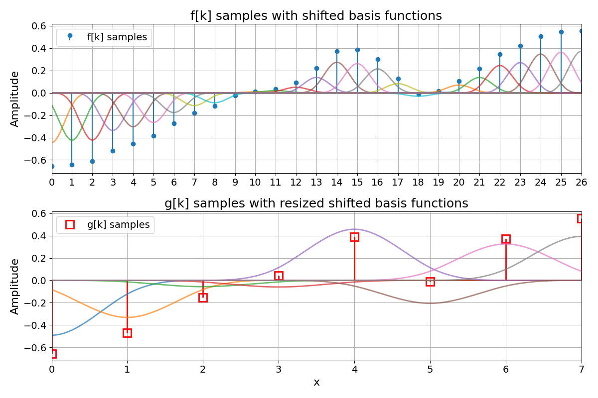
As a visual example, the following figure from Resample a 1D Spline has two rows. The top row shows the fine-grid samples \(f[k]\) together with their shifted basis functions \(\varphi(x - k)\) scaled by the coefficients \(c[k]\), illustrating the spline space \(V_1\). The bottom row shows the coarse samples \(g[k]\) together with their shifted basis functions \(\varphi(x/T - k)\) scaled by \(c_T[k]\), illustrating the spline space \(V_T\). In that example, \(\varphi = \beta^{3}\) is the cubic B-spline, and the coefficients \(c[k]\) and \(c_T[k]\) implement the standard interpolation scheme described in Spline Interpolation:

Resizing by Resampling

Suppose that the original signal \(f\) belongs to \(V_1\). For a given scale factor \(T\), we can form new samples on the scaled grid \(\Gamma_T\):

\[f_T[k] = f(Tk), \qquad k \in \mathbb{Z}.\]

These samples tell us how the original continuous spline \(f\) behaves at the new grid locations. The goal of resizing is to construct a new spline \(g_T \in V_T\) that is consistent with these samples and remains a good approximation of \(f\) in the continuous domain.

A natural way to define \(g_T\) is as an orthogonal projection of \(f\) onto \(V_T\) in \(L_2(\mathbb{R})\):

\[g_T = \underset{g \in V_T}{\arg\min} \,\|f - g\|_{L_2(\mathbb{R})}^2,\]

where the \(L_2(\mathbb{R})\) norm is given by

\[\|h\|_{L_2(\mathbb{R})}^2 = \int_{\mathbb{R}} \bigl|h(x)\bigr|^2 \,\mathrm{d}x.\]

This is the least-squares projection point of view: among all splines that live in \(V_T\) (on the grid \(\Gamma_T\)), we pick the one that is as close as possible to \(f\) in the \(L_2\) sense.

In this language:

• \(V_1\) is the input spline space (grid step 1),

• \(V_T\) is the output spline space (grid step \(T\)),

• and resizing is the operation \(V_1 \to V_T\) that maps the coefficients (or samples) of \(f\) to the coefficients \(c_T[k]\) of \(g_T\).

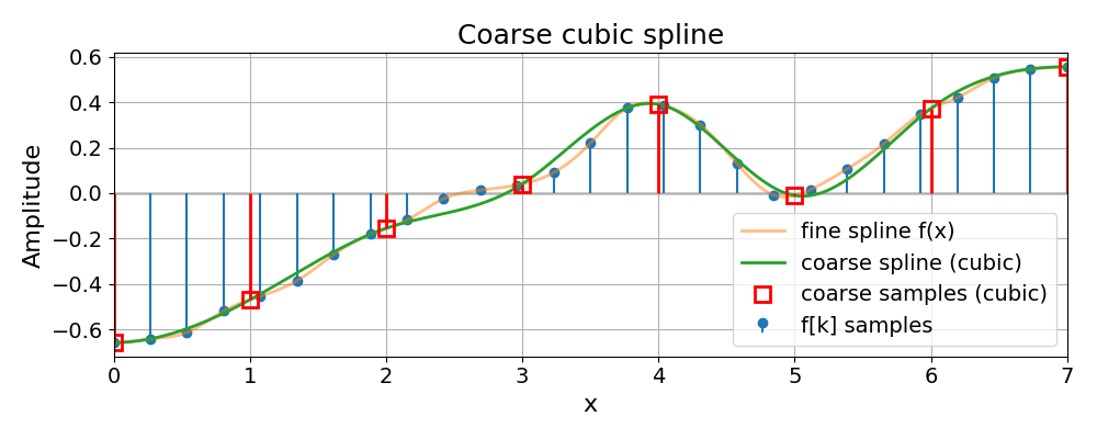
The next figure shows this operation in 1D: a fine spline \(f\) on \(V_1\) and its coarse counterpart \(g_T\) on the scaled grid \(\Gamma_T\), obtained by standard cubic interpolation.

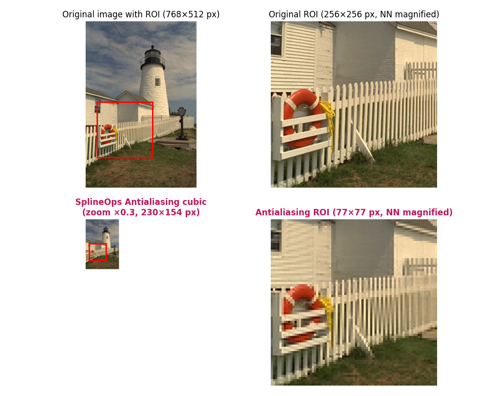
The following figure shows the same idea in 2D: an image is resampled from the fine grid to a coarser grid using standard cubic interpolation, illustrating how \(V_1 \to V_T\) looks in practice on real data.

Optimal Resizing by Least-Squares Projection

So far we have described elements of \(V_T\) by expanding them in terms of the shifted basis functions \(\varphi_{k,T}\):

\[g_T(x) = \sum_{k \in \mathbb{Z}} c_T[k]\,\varphi_{k,T}(x).\]

These functions \(\varphi_{k,T}\) play a synthesis role: they tell us how to reconstruct \(g_T\) once the coefficients \(c_T[k]\) are known. What remains is to explain how these coefficients are obtained from the input signal \(f\).

In the least-squares setting, this is done using a second family of functions \(\{\tilde{\varphi}_{k,T}\}_{k\in\mathbb{Z}}\), often called the analysis functions (also called dual-basis functions). They are chosen to be dual to the synthesis functions, in the sense of the biorthonormality relation

\[\bigl\langle \varphi_{k,T}, \tilde{\varphi}_{m,T} \bigr\rangle_{L_2(\mathbb{R})} = \delta_{km}, \qquad k,m \in \mathbb{Z},\]

where \(\delta_{km}\) is the Kronecker delta. Under mild conditions on \(\varphi\), this dual family exists and is unique. The least-squares projection \(g_T\) of \(f\) onto \(V_T\) can then be written as

\[g_T(x) = \sum_{k \in \mathbb{Z}} \bigl\langle f, \tilde{\varphi}_{k,T} \bigr\rangle_{L_2(\mathbb{R})} \,\varphi_{k,T}(x).\]

In other words, the least-squares coefficients \(c_T[k]\) are obtained by first analyzing \(f\) with the functions \(\tilde{\varphi}_{k,T}\) and then synthesizing with \(\varphi_{k,T}\):

\[c_T[k] = \bigl\langle f, \tilde{\varphi}_{k,T} \bigr\rangle_{L_2(\mathbb{R})}, \qquad k \in \mathbb{Z}.\]

The resized spline \(g_T\) is thus the least-squares (orthogonal) projection of \(f\) onto the spline space \(V_T\) [1].

Oblique Projection

For higher spline orders, the continuous-domain prefilters associated with the dual functions \(\tilde{\varphi}_{k,T}\) can become expensive to implement. A practical alternative is to replace the orthogonal (least-squares) projection by an oblique projection [2].

The idea is to keep the synthesis space \(V_T\) unchanged, i.e. the approximation is still written as

\[g_T^{\mathrm{obl}}(x) = \sum_{k \in \mathbb{Z}} d[k]\,\varphi_{k,T}(x),\]

but to compute the coefficients \(d[k]\) using a biorthonormal analysis family \(\{\psi_{k,T}\}_{k\in\mathbb{Z}}\) that typically belongs to a lower-degree spline space. In this case, the projection error is orthogonal to the analysis space spanned by \(\psi_{k,T}\), rather than to \(V_T\) itself, hence the term “oblique” projection.

When the analysis and synthesis spaces satisfy mild compatibility conditions, oblique projection retains the same approximation order as the least-squares projection and yields very similar quality in practice, while significantly reducing computational cost.

The 1D example below shows how the cubic-antialiasing preset implements this oblique projection: compared to plain cubic, the coarse spline is slightly smoother, but tracks the underlying fine spline more faithfully when downsampling.

The 2D example then shows the same effect on an image: the antialiasing preset suppresses Moiré and high-frequency artefacts in the downsampled ROI, while preserving the main structures and contrasts.

The Algorithm

At implementation level, resize follows the projection framework described above, but organized as a simple sequence of 1D operations applied axis by axis.

For a single axis, the algorithm works on one 1D line at a time:

1. Spline prefilter. The input samples along the line are first converted into spline coefficients using a stable recursive filter. After this step, the line represents a continuous spline in the sense of the previous sections, rather than just raw samples.

2. Optional projection prefilter. In antialiasing modes, a small number of discrete integrations and differences are applied to these coefficients. This realizes the least-squares / oblique projection prefilter from [1] and [2], and acts as a controlled low-pass filter when down-sampling. For pure interpolation this stage is skipped.

3. Boundary handling. Because real data are finite, each line is extended beyond its endpoints by symmetric or antisymmetric mirroring, depending on the spline degree. This produces a slightly longer “virtual” line on which the spline is evaluated, without introducing visible edge artefacts.

4. Resampling on the new grid. For the chosen zoom, the algorithm precomputes, once per axis, how every output position maps back to the original grid: which input coefficients contribute, and with which spline weights. During execution, each output sample is then obtained as a short weighted sum over that local window. This precomputation is what makes the method both accurate and efficient.

5. Projection tail (if enabled). When using antialiasing, the intermediate result is brought back from the analysis space to the desired spline model by applying the corresponding discrete differences and a final spline reconstruction on the output grid.

For N-dimensional data, this 1D scheme is applied separately along each axis in turn (a separable algorithm). All other axes are treated as batch dimensions, so the same 1D logic is reused for many lines, with a single precomputed plan per axis and zoom configuration.

Implementation

Internally, resize uses two cooperating backends:

• A compiled C++ core, wrapped as a small extension module. This is the primary implementation used in normal installations.

  For each axis, it:

  • builds a reusable 1D resampling plan that encodes, for every output position, which input coefficients contribute and with which spline weights (including boundary handling via mirrored extension),

  • constructs a single contiguous extended buffer per line that contains the mirrored input samples, so the inner loop only sees simple pointer arithmetic and dot products,

  • evaluates all spline sums in double precision, using small dense dot products that can exploit SIMD instructions (AVX2, AVX-512, NEON) when available,

  • and parallelizes over independent lines with a lightweight multithreading pool whenever the estimated workload is large enough.

  The plan is computed once per axis/zoom/degrees combination and then reused across all lines along that axis, which keeps the per-call overhead low even for large N-D arrays.

• A pure-NumPy fallback that mirrors the same 1D scheme at a higher level. It reshapes the data so that each line along the resized axis is contiguous, processes lines in batches, and uses vectorized gathers and reductions to apply the same precomputed weights. This backend is mainly intended for environments where the C++ extension cannot be built; it is numerically equivalent but typically slower.

Both backends perform all spline computations in 64-bit floating point; input and output arrays keep their original dtype (or a user-specified dtype), with casting only at the boundary of each axis pass.

Conceptually, resize is configured by three spline degrees:

• the interpolation degree, which sets the underlying spline model,

• the analysis degree, which controls the projection-based prefilter (for antialiasing; -1 means “no projection”),

• and the synthesis degree, which sets the spline model on the resized grid.

These degrees are exposed through the resize API via the method argument. There are two main families of presets.

Standard interpolation presets use no projection at all (analysis degree -1) and perform plain spline interpolation:

Spline degree standard interpolation presets in resize

Method	Interpolation degree	Analysis degree	Synthesis degree
"fast"	0	-1	0
"linear"	1	-1	1
"quadratic"	2	-1	2
"cubic"	3	-1	3

These are appropriate when you mainly want smooth interpolation and are not aggressively downsampling.

Antialiasing presets use an oblique projection with a lower analysis degree and a higher synthesis degree, and are designed for downsampling (and its inverse round-trip):

Spline degree antialiasing configuration in resize

Method	Interpolation degree	Analysis degree	Synthesis degree
"linear-antialiasing"	1	0	1
"quadratic-antialiasing"	2	1	2
"cubic-antialiasing"	3	1	3

Here, the synthesis degree matches the interpolation degree, defining the output spline model, while the lower analysis degree keeps the projection prefilter short, robust, and efficient, yet still very close to the ideal least-squares solution in [1] and [2].

Warning

Exact least-squares configurations, where the analysis and synthesis degrees are equal (for example, a cubic–cubic combination), require high-order discrete integration in this framework. For cubic splines, the theory calls for fourth-order integration: a running-sum operator applied four times in a row to implement the continuous prefilter. Each pass is stable in exact arithmetic, but in double precision they amplify tiny rounding errors, especially on long lines, which can lead to slow drift in the mean level and other visible artefacts. For this reason such configurations are not exposed as presets and are not recommended in routine use. The oblique antialiasing presets above avoid the problematic high-order integration while remaining very close in quality to the ideal least-squares projection.

Benchmarking

We compare our module resize against widely used interpolation libraries on realistic image resizing tasks, in these two examples:

• Benchmarking

• Benchmarking Plot

• Benchmarking Animation

Round-Trip ROI Benchmark

The first and third benchmark examples evaluate several images by:

1. downsampling with an image-specific zoom factor \(z < 1\),

2. upsampling back to the original size (round-trip),

3. measuring quality on a small region of interest (ROI) and reporting timing.

The compared methods include:

• scipy.ndimage.zoom (cubic),

• cv2.resize with INTER_CUBIC,

• PIL.Image.resize with BICUBIC resampling,

• skimage.transform.resize (cubic, with and without anti_aliasing),

• torch.nn.functional.interpolate (bicubic),

• our method resize() method="cubic" (standard cubic),

• our method resize() method="cubic-antialiasing" (projection-based antialiasing).

As a concrete example, we show a side-by-side round-trip comparison against PyTorch bicubic, which is a widely used high-quality baseline in modern pipelines. The animation sweeps a range of downsampling factors on an input image. The left column shows PyTorch; the right column shows SplineOps method="cubic-antialiasing".

Across the image test set, method="cubic-antialiasing" is designed to reduce downsampling artefacts by applying a projection-based low-pass step before decimation. In practice this typically shows up as:

• fewer Moiré / ripple patterns after downsampling,

• a recovered image that preserves local structure better after the round-trip,

• and smaller, less structured errors in the ROI (as seen in the error maps).

The accompanying benchmark scripts report the ROI metrics (SNR/MSE/SSIM) and round-trip timing for all methods and images.

Zoom-Sweep Benchmark

The second example uses a single Kodak image to run a 1D sweep of zoom factors \(0 < z < 2\). For each method and zoom, it:

• performs a forward and backward resize in float32,

• measures round-trip time, SNR and SSIM on the full image,

• plots these quantities as a function of \(z\) for both linear and cubic variants.

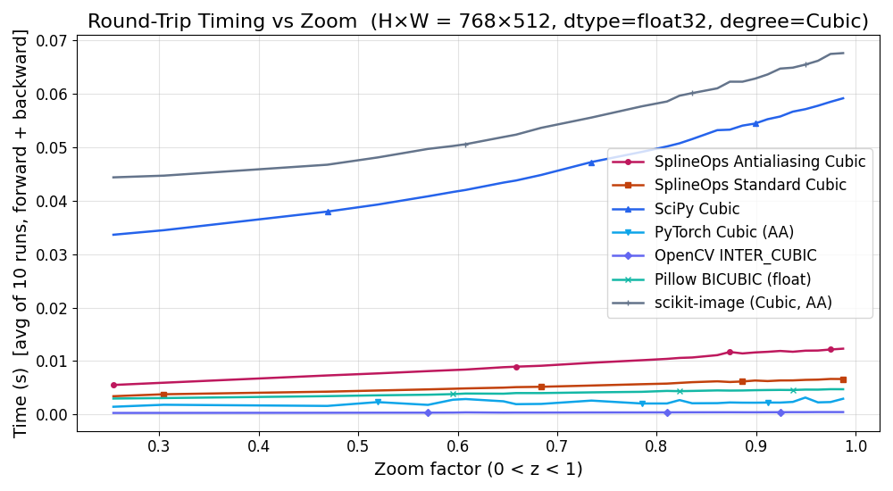
This provides an at-a-glance view of the quality–speed trade-off of each backend:

• OpenCV and PyTorch tend to be the fastest;

• SciPy and scikit-image tend to be the slowest;

• resize() sits in between, with method="cubic" methods matching the quality of traditional cubic/linear filters, and method="cubic-antialiasing" methods pushing quality (higher SNR/SSIM at small \(z\)) while remaining competitive in runtime.

The first plot below shows round-trip SNR vs zoom for cubic methods: resize() method="cubic-antialiasing" rises well above the other curves for strong downsampling and remains best for all resampling factors. In the zoomed version focusing on \(0 < z < 1\), it leads the next-best method by several decibels over a wide range of zoom factors, corresponding to a noticeably smaller reconstruction error:

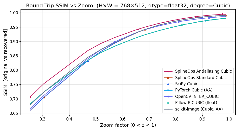
The next plot shows round-trip SSIM vs zoom for the same configuration: all methods converge near SSIM \(\approx 1\) around \(z = 1\), but resize() method="cubic-antialiasing" maintains a clear SSIM advantage for the more aggressive downsampling factors, meaning the recovered images preserve local structure better:

The last plot shows round-trip runtime vs zoom. It confirms that the antialiasing presets add only a modest overhead over the Standard ones, while still remaining competitive with other high-quality methods for a wide range of zoom factors. The zoomed version for \(0 < z < 1\) makes this clear in the practically most relevant regime (downsampling):

Resize Examples

• Resize Module 1D

• Resize Module 2D

• Standard Interpolation

• Antialiasing

• How Bad Aliasing Can Be

• Benchmarking

• Benchmarking Plot

• Benchmarking Animation

References

[1] (1,2,3)

A. Muñoz Barrutia, T. Blu, M. Unser, Least-Squares Image Resizing Using Finite Differences, IEEE Transactions on Image Processing, vol. 10, no. 9, pp. 1365-1378, September 2001.

[2] (1,2,3)

C. Lee, M. Eden, M. Unser, High-Quality Image Resizing Using Oblique Projection Operators, IEEE Transactions on Image Processing, vol. 7, no. 5, pp. 679–692, May 1998.