
All examples#
Explore the example gallery to see how to use the SplineOps library.
All real-world images used in these examples come from the Kodak image dataset, available at:
https://r0k.us/graphics/kodak/
We gratefully acknowledge the work of the author and curator of this dataset for making these images publicly available.
Spline Interpolation Examples#
Build continuous models from sampled data. Explore spline bases and boundary modes, then compare interpolation and resampling choices.
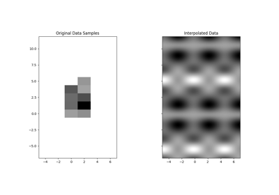
Build a continuous spline from 2-D samples and evaluate it on a finer grid.
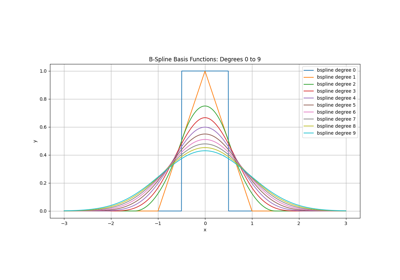
Explore B-spline, O-MOMS, and Keys bases, then combine shifted and weighted copies into continuous models.
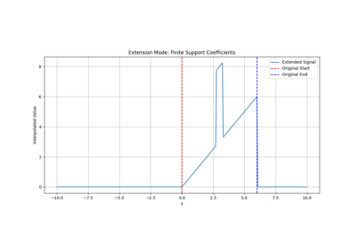
Compare zero, mirror, and periodic coefficient boundaries when evaluating a signal beyond its sampled interval.
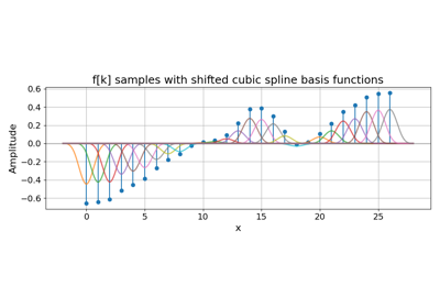
Reconstruct a 1-D signal with cubic and linear splines, and compare TensorSpline with Resize.
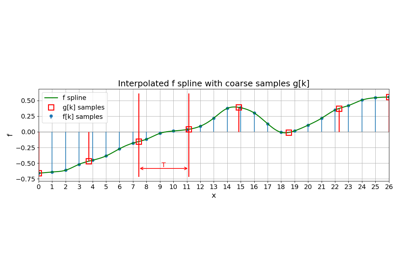
Move a continuous spline to a coarser sampling grid and inspect how its representation changes.
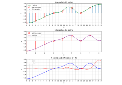
Compare spline reconstruction methods by expanding coarse samples and measuring error against the original model.
Resize Examples#
Resize signals and images with standard interpolation or projection antialiasing. Inspect fine detail, compare numerical quality, and measure runtime across zoom factors.
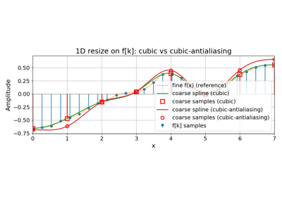
Compare standard cubic resizing and projection antialiasing on a 1-D signal.
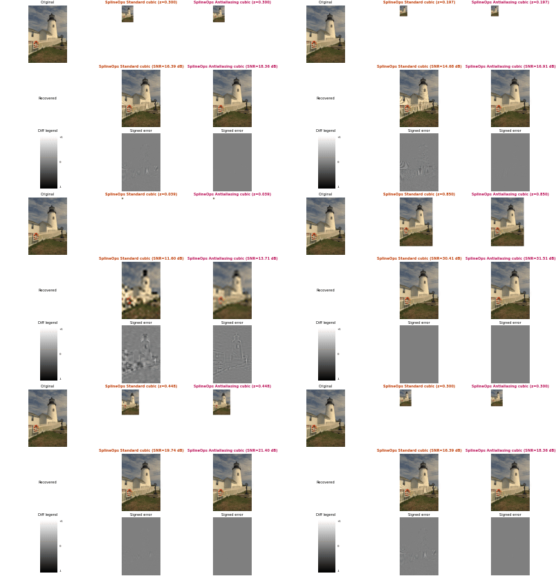
Resize an RGB image and use detail views and an animation to inspect aliasing.
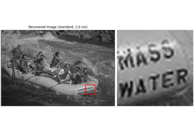
Compare SplineOps cubic interpolation with SciPy using matched image roundtrips and detail regions.
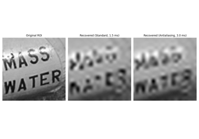
Compare image detail and reconstruction error after shrinking with and without projection antialiasing.
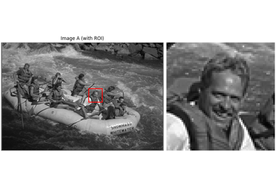
Use a deliberately mixed image to reveal how unfiltered downsampling can select misleading visual content.
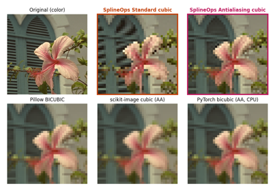
Compare resize methods across several Kodak images using detail views, reconstruction quality, and runtime.
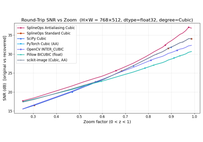
Sweep zoom factors and compare the speed and reconstruction quality of linear and cubic resize methods.
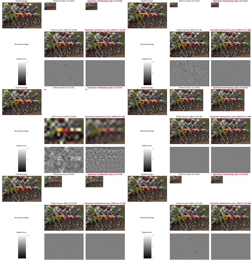
Animate image detail and reconstruction errors as the zoom factor changes across several test images.
Affine Examples#
Rotate images with spline interpolation. Start with a single transform, then use the animation to explore a full rotation and different spline degrees.
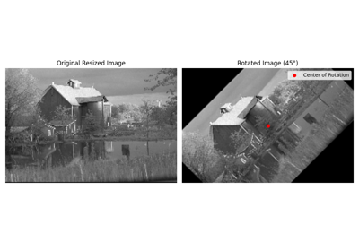
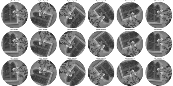
Animate a full image rotation and explore how spline degree affects interpolation.
Adaptive Regression Splines Examples#
Fit sparse piecewise-linear models to noisy observations. Compare fixed regularization strengths or watch the fit and knot count change in an animation.
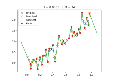
Adaptive Regression Splines Module
Fit sparse piecewise-linear models and compare how regularization changes the fit and knot count.
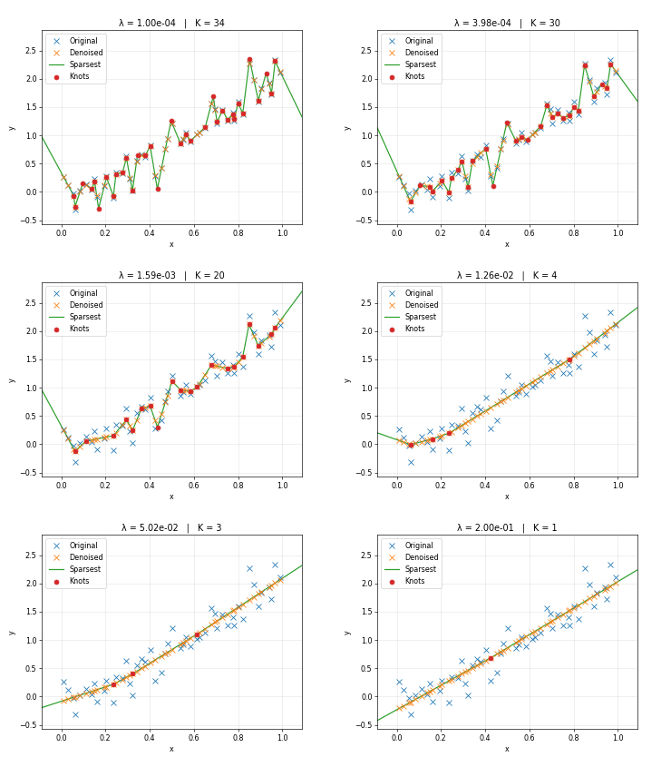
Animate the trade-off between data fidelity and knot sparsity while increasing regularization.
Smoothing Splines Examples#
Reduce noise in signals, images, and volumes. Compare fractional, periodic N-D, and recursive smoothers while keeping their different operators and boundaries explicit.
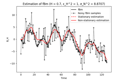
Generate a noisy fractional Brownian signal and recover its trend with a fractional smoothing spline.
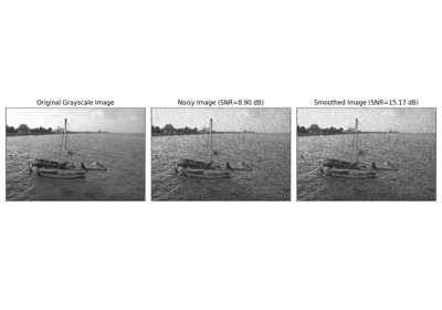
Denoise a grayscale image with periodic smoothing and compare image detail and signal-to-noise ratio.
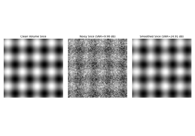
Smooth a noisy synthetic 3-D volume and compare central slices against its known clean signal.
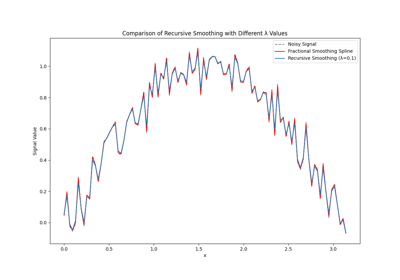
Compare regularization strengths in a recursive first-order smoother for noisy 1-D data.
Differentials Examples#
Turn image intensities into gradients, curvature, and orientation maps. Compare the meaning and appearance of each spline-based differential feature.
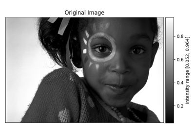
Visualize image gradients, the Laplacian, and Hessian features using spline-based derivatives.
Multiscale Examples#
Explore coarse-to-fine image representations. Build spline pyramids, inspect wavelet detail bands, and compare reconstruction across several levels.
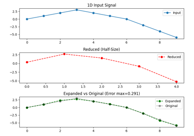
Reduce and expand 1-D signals and images, then compare several levels of a spline pyramid.
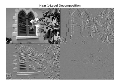
Inspect Haar detail bands at several scales and reconstruct the original image.
End-to-end workflows#
Combine reusable operators in complete pipelines. Share saved coefficients across rotations or write selected volume features into explicit output buffers.
Persist one frame and evaluate several affine geometries
Save one frame's spline coefficients and reuse them for several affine geometries.
Warp a volume and write selected differential features
Warp a synthetic 3-D volume and compute selected differential features into reusable output buffers.