Resize Module

We use the resize module to shrink and expand a 2D image.

You can download this example at the tab at right (Python script or Jupyter notebook.

Required Libraries

We import the required libraries, including NumPy for numerical computations, Matplotlib for plotting, and the custom resize function from the splineops package.

import numpy as np
import matplotlib.pyplot as plt
import requests
from io import BytesIO
from PIL import Image

from scipy.ndimage import zoom as ndi_zoom
from splineops.resize.resize import resize  # or your actual import path

Utility Functions

Adjustment of an image resolution using scipy and splineops.

def adjust_image_size_for_shrink(data, shrink_factor):
    """
    Adjust the image size so that after shrinking and re-expanding,
    the final dimensions match this 'adjusted image' exactly.

    Steps:
      1) We want H' * shrink_factor to be integer (same for W').
      2) Choose H' as nearest multiple of 1/shrink_factor to original H,
         similarly for W'.
      3) Use ndimage.zoom to resample to (H', W').
    """
    h, w = data.shape[:2]
    c = data.shape[2] if data.ndim == 3 else 1

    inv_s = 1.0 / shrink_factor

    # Determine new height
    new_h = round(round(h / inv_s) * inv_s)
    # Determine new width
    new_w = round(round(w / inv_s) * inv_s)

    new_h = max(new_h, 1)
    new_w = max(new_w, 1)

    # Scale factors for ndimage.zoom
    scale_factor_h = new_h / h
    scale_factor_w = new_w / w

    if c == 1:
        data_zoomed = ndi_zoom(data, (scale_factor_h, scale_factor_w), order=1)
    else:
        # For RGB: zoom each spatial dimension, but keep channels unchanged
        data_zoomed = ndi_zoom(data, (scale_factor_h, scale_factor_w, 1), order=1)

    return data_zoomed

def resize_image_splineops(data, zoom_factor, degree=3, extension_mode="mirror"):
    """
    Wrapper around splineops' resize function for a 3-channel (RGB) image.
    Assumes 'data' is float64 in [0, 1].
    """
    resized_channels = []
    for ch in range(data.shape[2]):
        resized_ch = resize(
            data[:, :, ch],
            zoom_factors=zoom_factor,
            degree=degree,
            modes=extension_mode,
            method="interpolation"
        )
        resized_channels.append(resized_ch)

    resized_image = np.stack(resized_channels, axis=-1)
    # Clip to [0,1], then convert to uint8
    resized_image = np.clip(resized_image, 0.0, 1.0)
    return (resized_image * 255.0).astype(np.uint8)

Basic Resizing Example

Load a simple 2D image, shrink and expand it using splineops interpolation.

# 1) Load and normalize the original image
url = 'https://r0k.us/graphics/kodak/kodak/kodim19.png'
response = requests.get(url)
img = Image.open(BytesIO(response.content))
data = np.array(img, dtype=np.float64)  # shape: (H, W, 3)
data_normalized = data / 255.0          # Convert to [0,1]

# 2) *Initially* shrink the image to reduce its overall size
initial_shrink_factor = 0.8
data_smaller = ndi_zoom(data_normalized, (initial_shrink_factor, initial_shrink_factor, 1), order=1)

# 3) Next, adjust the now-smaller image so that our subsequent shrink-and-expand
#    steps (by shrink_factor below) will match the final shape exactly.
shrink_factor = 0.3
adjusted_data = adjust_image_size_for_shrink(data_smaller, shrink_factor)
adjusted_data_uint8 = (adjusted_data * 255).astype(np.uint8)

# 4) Shrink the adjusted image via splineops
shrunken_image = resize_image_splineops(
    adjusted_data,
    zoom_factor=shrink_factor,
    degree=3,
    extension_mode="mirror"
)

# 5) Place the shrunken image onto a white canvas the size of the adjusted image
H_adj, W_adj, _ = adjusted_data_uint8.shape
canvas_shrunken = np.ones((H_adj, W_adj, 3), dtype=np.uint8) * 255  # white background
H_shr, W_shr, _ = shrunken_image.shape
canvas_shrunken[:H_shr, :W_shr, :] = shrunken_image

# 6) Expand the shrunken image back to the adjusted image dimensions
expanded_image = resize_image_splineops(
    shrunken_image.astype(np.float64) / 255.0,  # re-normalize to [0,1]
    zoom_factor=1.0 / shrink_factor,
    degree=3,
    extension_mode="mirror"
)

# 7) Plot the three images in one figure, stacked vertically
#    to achieve a large, clear display. We also increase font sizes.
plt.rcParams.update({
    "font.size": 14,     # Base font size
    "axes.titlesize": 18,  # Title font size
    "axes.labelsize": 16,  # Label font size
    "xtick.labelsize": 14,
    "ytick.labelsize": 14
})

fig, axes = plt.subplots(3, 1, figsize=(8, 18))

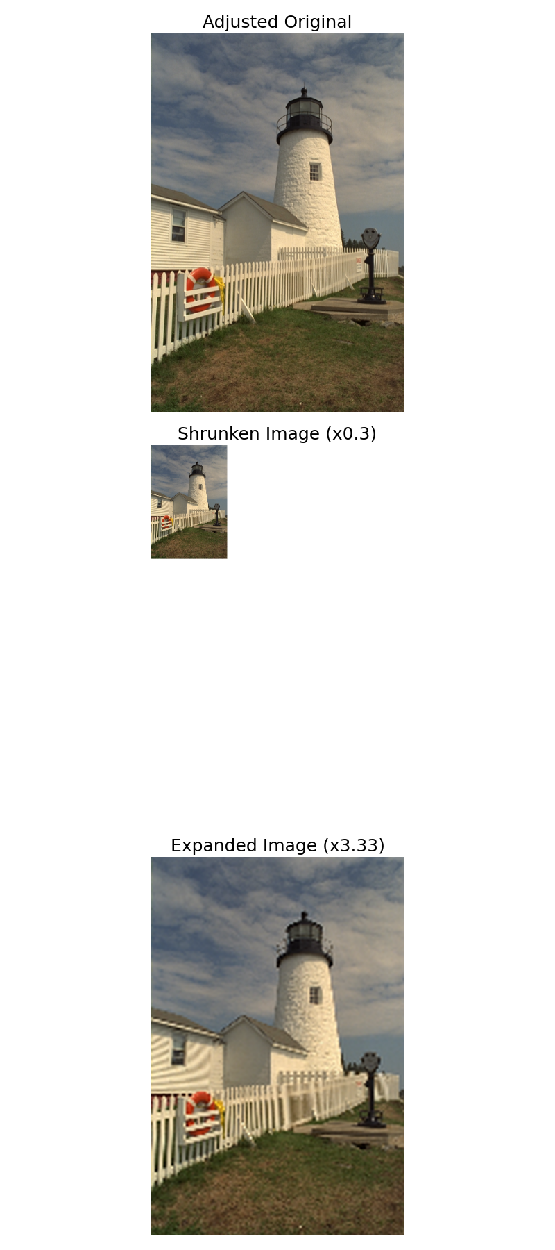
axes[0].imshow(adjusted_data_uint8)
axes[0].set_title("Adjusted Original")
axes[0].axis("off")

axes[1].imshow(canvas_shrunken)
axes[1].set_title(f"Shrunken Image (x{shrink_factor})")
axes[1].axis("off")

axes[2].imshow(expanded_image)
axes[2].set_title(f"Expanded Image (x{1/shrink_factor:.2f})")
axes[2].axis("off")

plt.tight_layout()
plt.show()

Aliasing

Note that we observe aliasing in the expanded image.

Aliasing: When we shrink an image below the Nyquist limit for its higher-frequency details, those details cannot be represented adequately at the smaller sampling rate. As a result, they become “aliased”—folded back into lower-frequency components. When we then re-expand the image, these aliased components manifest as artificial wave-like or Moiré patterns, since the original high-frequency content is irretrievably lost in the shrinking step.

In practice, one might mitigate aliasing by pre-filtering or low-pass filtering before downsampling, but here we demonstrate straightforward interpolation, which can reveal aliasing artifacts in areas with fine detail.