Displaying signal extension modes

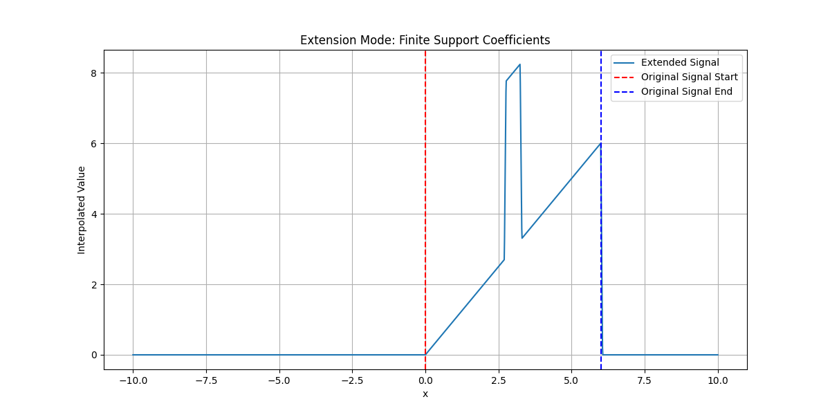
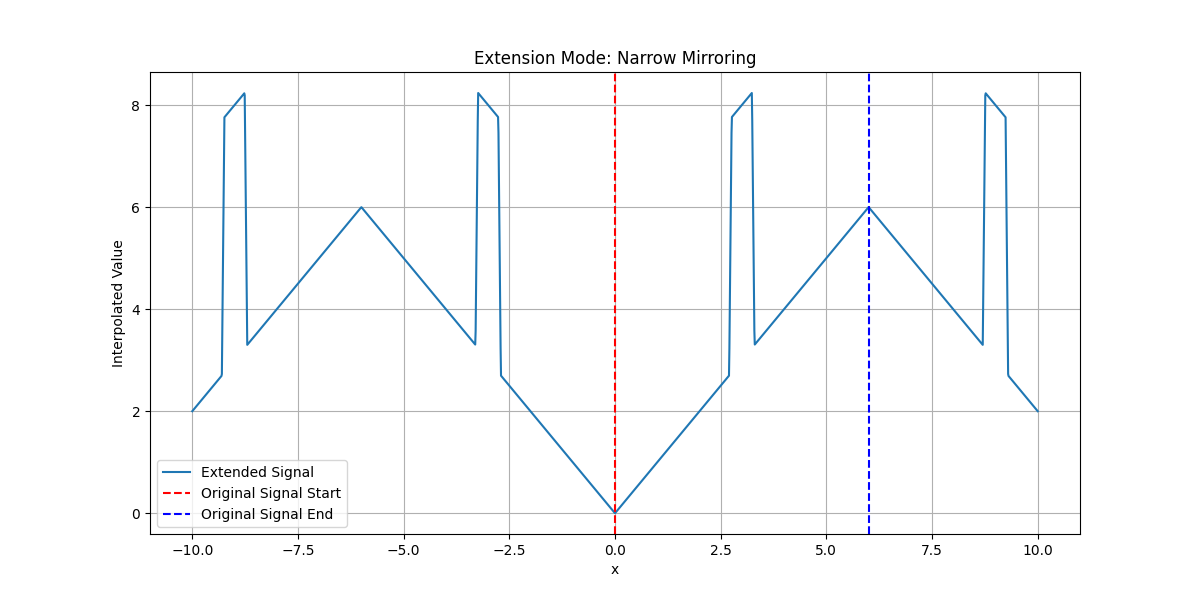
This example shows current extension modes finite support coefficients and narrow mirroring.

Imports

Import the necessary libraries and utility functions.

import numpy as np
import matplotlib.pyplot as plt
from splineops.interpolate.tensorspline import TensorSpline

Function to create non-continuous signal

Create a signal that is mostly linear but introduces a “bump” at an arbitrary location.

def create_signal_with_bump(x_values, bump_location=3, bump_width=0.5, bump_height=5):
    linear_part = x_values  # Linear function: f(x) = x
    bump = np.where(
        (x_values > (bump_location - bump_width / 2))
        & (x_values < (bump_location + bump_width / 2)),
        bump_height,
        0,
    )
    return linear_part + bump

Function to plot extension modes for signal

Define a helper function to plot extension modes using the non-continuous function.

def plot_extension_modes_for_bump_function(mode_name, x_values, title):
    plt.figure(figsize=(12, 6))

    # Create the signal with a bump
    data = create_signal_with_bump(x_values)

    # Create TensorSpline instance
    tensor_spline = TensorSpline(
        data=data, coordinates=(x_values,), bases="linear", modes=mode_name
    )

    # Define the extended evaluation grid (from -10 to 10)
    eval_x_values = np.linspace(-10, 10, 2000)
    eval_coords = (eval_x_values,)

    # Evaluate the tensor spline
    extended_data = tensor_spline.eval(coordinates=eval_coords)

    # Plot the results
    plt.plot(eval_x_values, extended_data, label="Extended Signal")

    # Add vertical lines at the boundaries of the original signal
    plt.axvline(
        x=x_values[0], color="red", linestyle="--", label="Original Signal Start"
    )
    plt.axvline(
        x=x_values[-1], color="blue", linestyle="--", label="Original Signal End"
    )

    plt.title(title)
    plt.xlabel("x")
    plt.ylabel("Interpolated Value")
    plt.grid(True)
    plt.legend()
    plt.show()

Define x range

x_values = np.linspace(0, 6, 101)  # Use 101 points to ensure 0 (middle) is included

Plot for finite support coefficients

plot_extension_modes_for_bump_function(
    mode_name="zero",  # Finite Support Coefficients is represented by "zero"
    x_values=x_values,
    title="Extension Mode: Finite Support Coefficients",
)

Plot for narrow mirroring

plot_extension_modes_for_bump_function(
    mode_name="mirror",  # Narrow Mirroring is represented by "mirror"
    x_values=x_values,
    title="Extension Mode: Narrow Mirroring",
)