Differentials#
Overview#
The differentials module in SplineOps provides a collection of algorithms for the computation of image differentials based on cubic B-spline interpolation [1], [2]. By modeling a grayscale image as a continuous function reconstructed from its discrete samples, the module enables the accurate computation of derivatives. It offers several operations such as
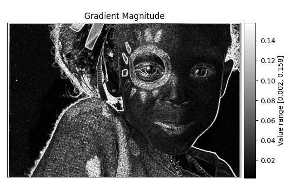
Gradient Magnitude: the local rate of change of the intensity;
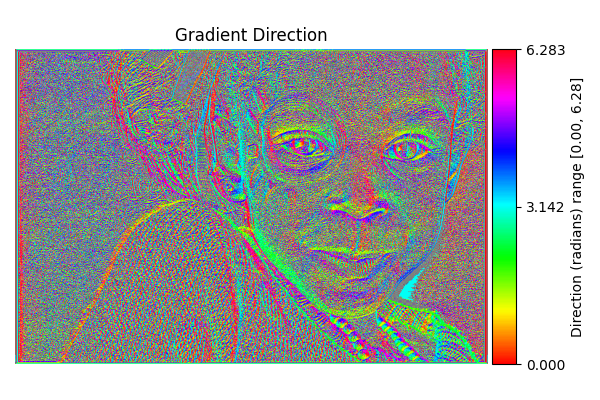
Gradient Direction: the direction along which the intensity changes most;
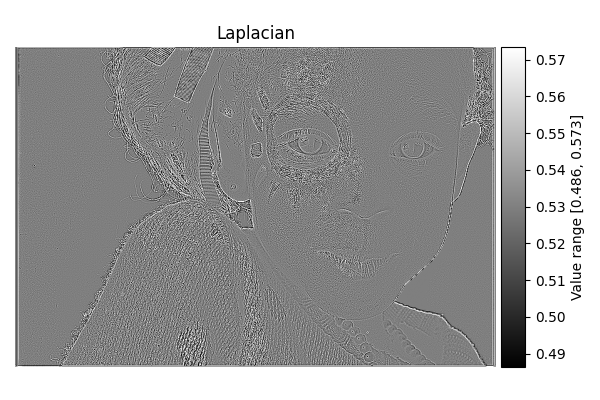
Laplacian:the sum of second-order derivatives;
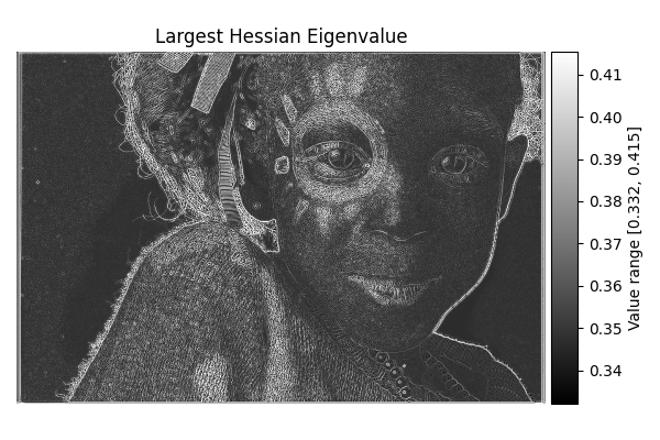
Largest Hessian Eigenvalue: the maximal curvature;
Smallest Hessian Eigenvalue: the minimal curvature; and
Hessian Orientation: the principal orientation of the curvature.
Image Representation#
A grayscale image is modeled as the continuous function
where \(\varphi(x_1,x_2)\) is defined as the tensor-product cubic B‑spline
This formulation allows one to compute exact derivatives of the image by first determining the spline coefficients \(c[k_1,k_2]\).
Differentiation Operations#
Based on the spline representation, the module computes several differential operators. We define
Gradient Magnitude: Computed as the Euclidean norm of the first derivatives
\[\|\pmb{\nabla}f(x,y)\| = \sqrt{\bigl(f_1\bigr)^2 + \bigl(f_2\bigr)^2}.\]Gradient Direction: The direction of the gradient is given by
\[\theta(x,y) = \arctan\!\Bigl(\tfrac{f_2}{f_1}\Bigr).\]Laplacian: A second-order operator that highlights regions of rapid intensity change as
\[\Delta f(x,y) = f_{11} + f_{22}.\]Largest Hessian Eigenvalue: The maximal eigenvalue of the Hessian matrix is given by
\[\lambda_{\text{max}} = \tfrac12\Bigl(f_{11} + f_{22} + \sqrt{4f_{12}^2 + (f_{11} - f_{22})^2}\Bigr).\]Smallest Hessian Eigenvalue: The minimal eigenvalue of the Hessian matrix is given by
\[\lambda_{\text{min}} = \tfrac12\Bigl(f_{11} + f_{22} - \sqrt{4f_{12}^2 + (f_{11} - f_{22})^2}\Bigr).\]Hessian Orientation: This operation returns the orientation that corresponds to the maximal second derivative, as
\[\theta_H(x,y) = \pm \tfrac12 \arccos\!\Bigl(\tfrac{f_{11} - f_{22}}{\sqrt{4f_{12}^2 + (f_{11}-f_{22})^2}}\Bigr),\]where the sign is determined by the sign of the cross derivative \(f_{12}\).
Implementation Details#
The Differentials class implements these operations as follows: the input image is provided by its samples. We assume it to be a cubic B-spline and first determine its interpolation coefficients. The differential-based computations that we perform are then perfectly consistent with this continuously defined function. We finally build the output image by sampling the ideal, continuously defined intermediate result.
The following figure, taken from Differentials Module, shows some of these differential maps (gradient magnitude, gradient direction, Laplacian and Hessian-based quantities).