
Adaptive Regression Splines#
Overview#
The adaptive regression splines module in SplineOps performs one-dimensional regression with total-variation (TV) regularisation on the second derivative [1]. Because TV is measured with the measure norm (denoted \(\|\cdot\|_{\mathcal{M}}\)), solutions are piecewise-linear splines that use few knots, giving very compact models.
Key Features#
Produces piecewise-linear solutions with few knots.
Provides a two-step denoising and sparsification implementation.
Works for both interpolation (exact fit) and regression (noisy data).
These properties are valuable in machine learning (where sparsity improves generalisation) and in signal processing (where interpretability matters). In 1D, the method is closely related to rectified linear unit (ReLU) neural networks, which also create piecewise-linar functions, but here we obtain the sparsest possible representation directly.
Mathematical Background#
Problem Formulation#
where
the regularization parameter \(\lambda>0\) balances fidelity and sparsity;
the operator \(\mathrm{D}^2\) is the second derivative;
the norm \(\|\cdot\|_{\mathcal{M}}\) is the total variation (TV) norm on measures, promoting sparse second derivatives.
This is the generalised Beurling LASSO (g-BLASSO): it extends the classical LASSO (\(L^1\) regularisation on vectors) and the Beurling LASSO (BLASSO, \(L^1\) on measures) by inserting the linear operator \(\mathrm{D}^2\).
Representer Theorem#
A solution of the g-BLASSO has the form
where
\(b_0,b_1\in\mathbb{R}\) describe the global trend;
\((x-\tau_k)_+\) is a shifted ReLU function;
the number \(K\) satisfies \(K\le M-2\), so only few knots appear.
Uniqueness and Sparsity#
The g-BLASSO may admit multiple solutions. The method in [1] characterizes a sparsest solution; this implementation follows that construction and is kept experimental while its numerical behavior is validated beyond the current deterministic synthetic cases.
Algorithm#
The solver uses two stages*:
Data fitting: solve a discrete \(L^1\)-regularised problem to obtain \(y_\lambda\) (each ADMM iteration costs \(\mathcal{O}(M)\) and the residual decreases like \(\mathcal{O}(1/n)\)).
Sparsification: in exactly \(\mathcal{O}(M)\) time, extract the spline with the fewest knots.
*Stage 2 is linear-time; stage 1 is linear per iteration.
Advantages and Applications#
Compact representation: redundant numerical knots are pruned while the reconstructed piecewise-linear function is checked at the samples.
Exact interpolation: with \(\lambda=0\), the method finds the least angular spline through every point.
Segmented regression: ideal for interpretable fits in finance, epidemiology, etc.
ReLU connection: in 1-D this outperforms naïve ReLU networks in terms of parameter count.
Regularisation Parameter#
Choosing \(\lambda\):
Small \(\lambda\) → exact or near-exact interpolation (risk of over-fit).
Large \(\lambda\) → smoother, eventually linear.
Practical tip: run the solver on a grid of \(\lambda\) values and plot sparsity vs. data-fidelity (e.g., root-MSE) to pick a balanced point.
For such a sweep, splineops.adaptive_regression_splines.DenoisingPlan
factorizes the fixed x/rho system once. Observations and regularization
strength may change between solves:
from splineops.adaptive_regression_splines import DenoisingPlan

plan = DenoisingPlan(x, rho=1e-3)
solutions = [plan.solve(y, lamb=value) for value in lambda_values]
This removes repeated sparse factorization but does not make the iterative ADMM
work disappear. x must stay strictly increasing and rho is fixed by
the plan; construct another plan when either changes. Zero regularization and
the linear-regression limit still use their direct branches.
For an ordered sweep on one signal, solve_path uses controlled warm starts:
solutions, diagnostics = plan.solve_path(
    y,
    lambda_values,
    return_diagnostics=True,
)
Iteration state is local to that call. Repeated calls therefore remain
deterministic and the plan stays safe from hidden cross-call state. Nearby
penalties often require fewer iterations, but this is not a guaranteed speedup;
the diagnostics expose the actual result. retained_array_bytes is a lower
bound covering known NumPy/SciPy sparse arrays, excluding opaque solver-factor
storage.
Convergence diagnostics#
denoise_y keeps its historical array return by default. Set
return_diagnostics=True to receive a DenoisingDiagnostics record with
the iteration count, convergence flag, and final primal and dual residuals:
from splineops.adaptive_regression_splines import denoise_y

denoised, diagnostics = denoise_y(
    x,
    y,
    lamb=1e-3,
    rho=1e-3,
    return_diagnostics=True,
)
The record makes an exhausted iteration budget visible instead of implying
convergence. Zero regularization and the linear-regression limit are solved
without ADMM and report zero iterations. rho affects convergence speed;
for difficult cases it should be tuned together with \(\lambda\).
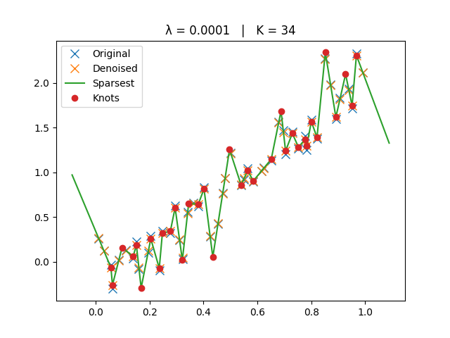
The figure below, taken from Adaptive Regression Splines Module, shows noisy 1D data (crosses), the TV-denoised samples, and the sparsest piecewise-linear spline for a given value of \(\lambda\), together with its knot locations.
Lambda Sweep Animation#
Here a more comprehensive animation exported from the example Lambda Sweep Animation, trying different values of \(\lambda\).