Affine

Overview

The affine module in SplineOps provides affine geometric transforms for 2D or 3D data arrays using spline interpolation. At the moment it exposes a single helper, rotate(), which rotates data around a specified axis and center. Such operations are widely used in image processing, computer graphics, and scientific computing [1].

2D Rotation

In 2D space, a point of coordinates \((x, y)\) can be rotated around a center point \((x_\mathrm{c}, y_\mathrm{c})\) by an angle \(\theta\) (in radians) using the rotation matrix.

\[\begin{split}\begin{pmatrix} x' \\ y' \end{pmatrix} = \begin{pmatrix} \cos\theta & -\sin\theta \\ \sin\theta & \cos\theta \end{pmatrix} \begin{pmatrix} x - x_\mathrm{c} \\ y - y_\mathrm{c} \end{pmatrix} + \begin{pmatrix} x_\mathrm{c} \\ y_\mathrm{c} \end{pmatrix}\end{split}\]

Here, \((x', y')\) are the coordinates of the rotated point.

3D Rotation

For 3D data, a point \(\mathbf{v} = (x, y, z)\) can be rotated around an arbitrary axis defined by a unit vector \(\mathbf{u} = (u_\mathrm{x}, u_\mathrm{y}, u_\mathrm{z})\) by an angle \(\theta\) using Rodrigues’ rotation formula

\[\mathbf{v}' = \mathbf{v} \cos\theta + (\mathbf{u} \times \mathbf{v}) \sin\theta + \mathbf{u} \left( \mathbf{u} \cdot \mathbf{v} \right) (1 - \cos\theta)\]

Alternatively, the rotation can be expressed with the rotation matrix

\[\begin{split}\mathbf{R} = \begin{pmatrix} \cos\theta + u_{\mathrm{x}}^2\,(1 - \cos\theta) & u_{\mathrm{x}}\,u_{\mathrm{y}}\,(1 - \cos\theta) - u_{\mathrm{z}}\,\sin\theta & u_{\mathrm{x}}\,u_{\mathrm{z}}\,(1 - \cos\theta) + u_{\mathrm{y}}\,\sin\theta \\[6pt] u_{\mathrm{y}}\,u_{\mathrm{x}}\,(1 - \cos\theta) + u_{\mathrm{z}}\,\sin\theta & \cos\theta + u_{\mathrm{y}}^2\,(1 - \cos\theta) & u_{\mathrm{y}}\,u_{\mathrm{z}}\,(1 - \cos\theta) - u_{\mathrm{x}}\,\sin\theta \\[6pt] u_{\mathrm{z}}\,u_{\mathrm{x}}\,(1 - \cos\theta) - u_{\mathrm{y}}\,\sin\theta & u_{\mathrm{z}}\,u_{\mathrm{y}}\,(1 - \cos\theta) + u_{\mathrm{x}}\,\sin\theta & \cos\theta + u_{\mathrm{z}}^2\,(1 - \cos\theta) \end{pmatrix}\end{split}\]

The rotated point is calculated as

\[\begin{split}\begin{pmatrix} x' \\ y' \\ z' \end{pmatrix} = \mathbf{R} \begin{pmatrix} x - x_\mathrm{c} \\ y - y_\mathrm{c} \\ z - z_\mathrm{c} \end{pmatrix} + \begin{pmatrix} x_\mathrm{c} \\ y_\mathrm{c} \\ z_\mathrm{c} \end{pmatrix}\end{split}\]

Affine Transformation by Resampling

The rotated coordinates may not coincide with the original data grid, so spline interpolation is employed for the resampling of the rotated data. The approach documented here uses standard interpolation, which leverages tensor-product B-splines for smooth, accurate results across multiple dimensions while minimizing artifacts like aliasing. The process asks one to first recenter the coordinates so that the rotation center coincides with the origin, then to apply the appropriate 2D or 3D rotation matrix to the recentered coordinates, followed by a translation of the rotated recentered coordinates back to their original reference frame, to compensate for the recentering step, and finally to use spline interpolation to determine the data values at these new positions.

Note

The geometry of the transform (center, axis, angle) is identical across methods; what changes is the spline used for resampling. Different spline degrees trade sharpness for smoothness (e.g., degree 0/nearest → blocky but fast; degree 1/linear → slight blur; degree 3/cubic → smoother, higher-quality edges).

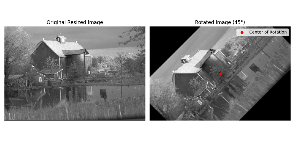
The following figure from Rotate Image shows an image rotated around a user-defined center using cubic interpolation. The red marker indicates the chosen center of rotation.

Rotation Animation

Here a more comprehensive animation exported from the example Rotation Animation, using different values of rotation angles and spline degrees.

Rotate Examples

• Rotate Image

• Rotation Animation

References

[1]

M. Unser, Splines: A Perfect Fit for Signal and Image Processing, IEEE-SPS best paper award, IEEE Signal Processing Magazine, vol. 16, no. 6, pp. 22-38, November 1999.