Usage of the Class TensorSpline

Showcase TensorSpline class basic functionality.

You can download this example at the tab at right (Python script or Jupyter notebook.

Imports

Import the necessary libraries and modules.

import numpy as np
import matplotlib.pyplot as plt
from splineops.interpolate.tensorspline import TensorSpline
from splineops.bases.utils import create_basis

Data Preparation

General configuration and sample data.

dtype = "float32"

nx, ny = 2, 5
xmin, xmax = 0, 2.0
ymin, ymax = 0, 5.0
xx = np.linspace(xmin, xmax, nx, dtype=dtype)
yy = np.linspace(ymin, ymax, ny, dtype=dtype)
coordinates = xx, yy
prng = np.random.default_rng(seed=5250)
data = prng.standard_normal(size=tuple(c.size for c in coordinates))
data = np.ascontiguousarray(data, dtype=dtype)

TensorSpline Setup

Configure bases and modes for the TensorSpline.

bases = "bspline3"
modes = "mirror"
tensor_spline = TensorSpline(data=data, coordinates=coordinates, bases=bases, modes=modes)

Evaluation Coordinates

Define evaluation coordinates to extend and oversample the original grid.

dx = (xx[-1] - xx[0]) / (nx - 1)
dy = (yy[-1] - yy[0]) / (ny - 1)
pad_fct = 1.0
px = pad_fct * nx * dx
py = pad_fct * ny * dy
eval_xx = np.linspace(xx[0] - px, xx[-1] + px, 100 * nx)
eval_yy = np.linspace(yy[0] - py, yy[-1] + py, 100 * ny)
eval_coords = eval_xx, eval_yy

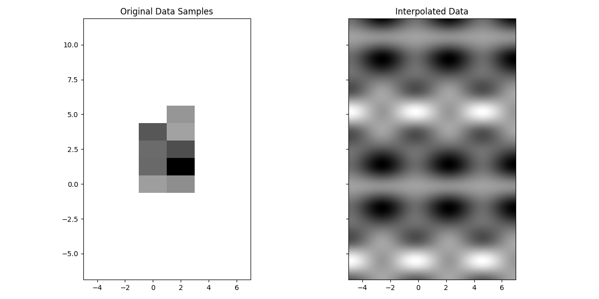
Interpolation and Visualization

Perform interpolation and visualize the original and interpolated data.

data_eval = tensor_spline(coordinates=eval_coords)

extent = [xx[0] - dx / 2, xx[-1] + dx / 2, yy[0] - dy / 2, yy[-1] + dy / 2]
eval_extent = [
    eval_xx[0] - dx / 2,
    eval_xx[-1] + dx / 2,
    eval_yy[0] - dy / 2,
    eval_yy[-1] + dy / 2,
]

fig, axes = plt.subplots(nrows=1, ncols=2, figsize=(12, 6), sharex="all", sharey="all")
axes[0].imshow(data.T, extent=extent, cmap="gray", aspect="equal")
axes[0].set_title("Original Data Samples")
axes[1].imshow(data_eval.T, extent=eval_extent, cmap="gray", aspect="equal")
axes[1].set_title("Interpolated Data")
plt.tight_layout()
plt.show()

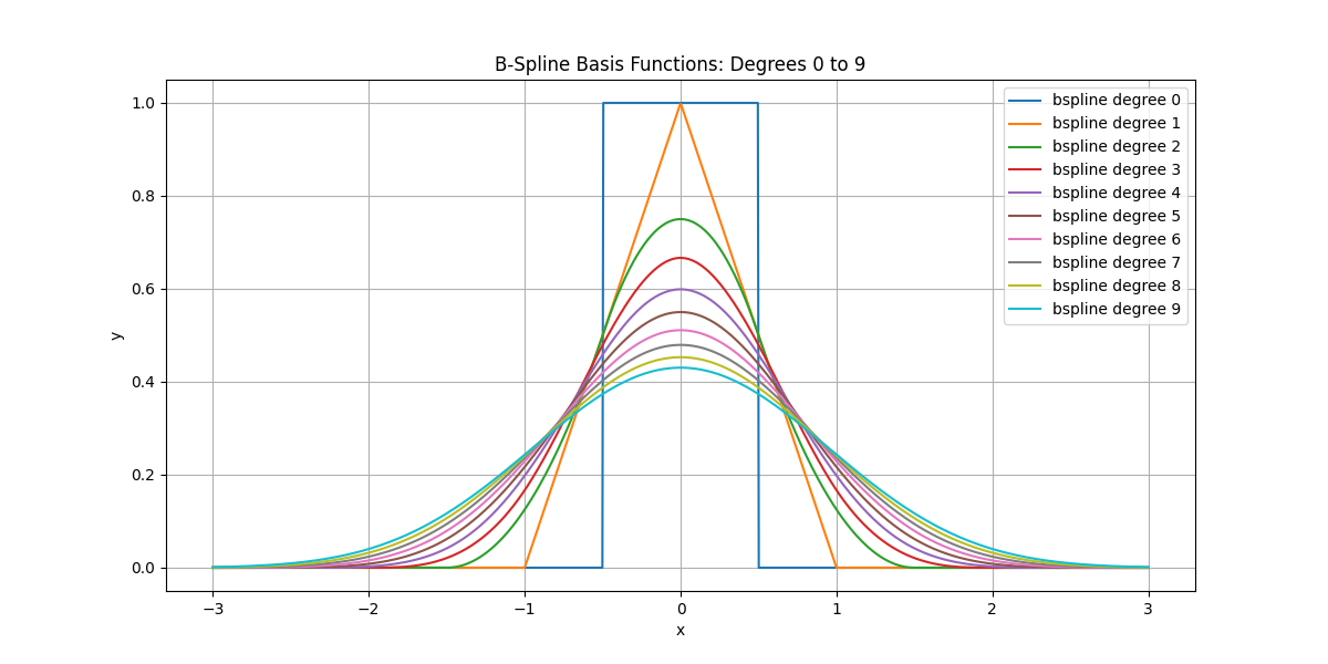
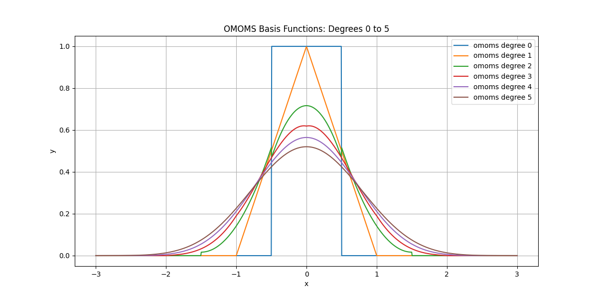
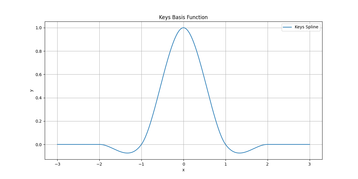
Plotting of Spline Bases

Define a helper function to visualize the spline bases.

x_values = np.linspace(-3, 3, 1000) # Define x range

def plot_bases(names, x_values, title):
    plt.figure(figsize=(12, 6))
    for name in names:
        if name == "keys":
            readable_name = "Keys Spline"
        else:
            name_parts = name.split("-")
            readable_name = f"{name_parts[0][:-1]} degree {name_parts[0][-1]}"
        y_values = create_basis(name).eval(x_values)
        plt.plot(x_values, y_values, label=readable_name)

    plt.title(title)
    plt.xlabel("x")
    plt.ylabel("y")
    plt.grid(True)
    plt.legend()
    plt.show()

Plot B-Spline Bases

Plot B-spline basis functions for degree 0 to 9.

plot_bases(
    names=[f"bspline{i}" for i in range(10)],
    x_values=x_values,
    title="B-Spline Basis Functions: Degrees 0 to 9",
)

Plot OMOMS Bases

Plot OMOMS basis functions for degree 0 to 5.

plot_bases(
    names=[f"omoms{i}" for i in range(6)],
    x_values=x_values,
    title="OMOMS Basis Functions: Degrees 0 to 5",
)

Plot Keys Basis

Plot the Keys basis function.

plot_bases(
    names=["keys"],
    x_values=x_values,
    title="Keys Basis Function",
)

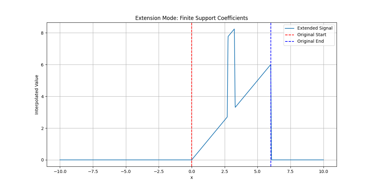
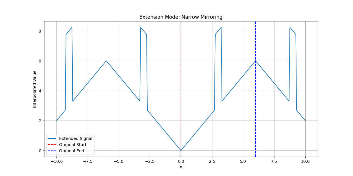
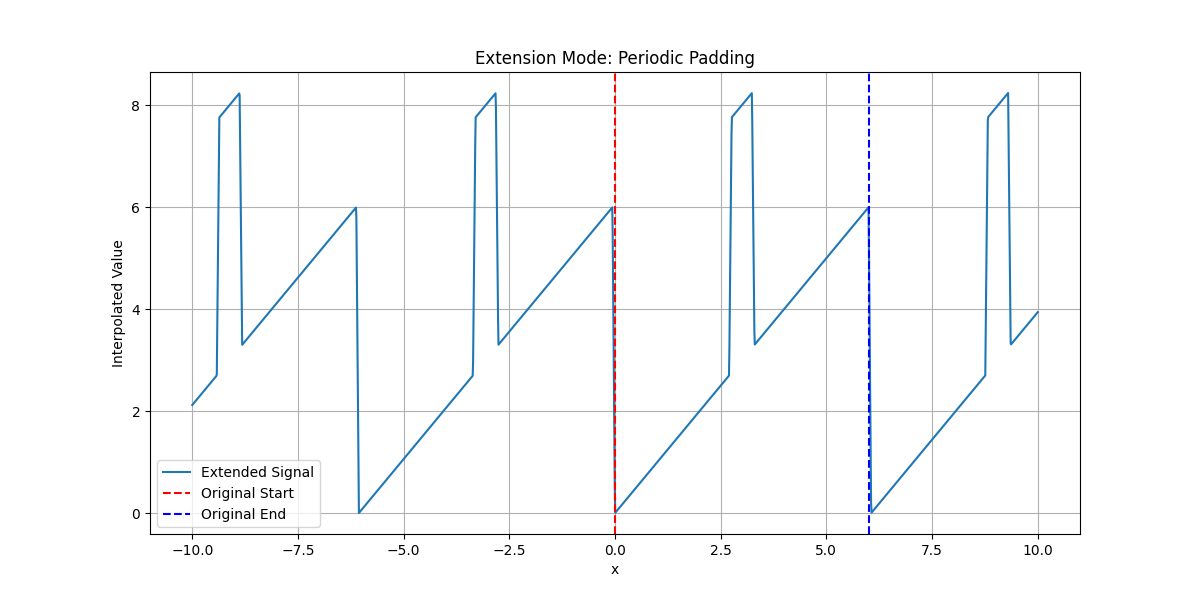
Plot Extension Modes

Visualize how the extension modes allow one to control the values that a signal is assumed to take outside of its original domain.

# Generate a signal that is mostly linear but includes a "bump."

x_values = np.linspace(0, 6, 101) # Define x range

def create_signal_with_bump(x_values, bump_location=3, bump_width=0.5, bump_height=5):
    linear_part = x_values
    bump = np.where(
        (x_values > (bump_location - bump_width / 2))
        & (x_values < (bump_location + bump_width / 2)),
        bump_height,
        0,
    )
    return linear_part + bump

def plot_extension_modes_for_bump_function(mode_name, x_values, title):
    plt.figure(figsize=(12, 6))
    data = create_signal_with_bump(x_values)
    tensor_spline = TensorSpline(
        data=data, coordinates=(x_values,), bases="linear", modes=mode_name
    )
    eval_x_values = np.linspace(-10, 10, 2000)
    extended_data = tensor_spline.eval(coordinates=(eval_x_values,))
    plt.plot(eval_x_values, extended_data, label="Extended Signal")
    plt.axvline(x=x_values[0], color="red", linestyle="--", label="Original Start")
    plt.axvline(x=x_values[-1], color="blue", linestyle="--", label="Original End")
    plt.title(title)
    plt.xlabel("x")
    plt.ylabel("Interpolated Value")
    plt.grid(True)
    plt.legend()
    plt.show()

Finite-Support Coefficients

plot_extension_modes_for_bump_function(
    mode_name="zero",
    x_values=x_values,
    title="Extension Mode: Finite Support Coefficients",
)

Narrow Mirroring

plot_extension_modes_for_bump_function(
    mode_name="mirror",
    x_values=x_values,
    title="Extension Mode: Narrow Mirroring",
)

Periodic Padding

plot_extension_modes_for_bump_function(
    mode_name="periodic",
    x_values=x_values,
    title="Extension Mode: Periodic Padding",
)

GPU Support

We leverage the GPU for TensorSpline if cupy is installed. If cupy is not available, we skip this section.

try:
    import cupy as cp
    HAS_CUPY = True
except ImportError:
    HAS_CUPY = False

if not HAS_CUPY:
    print("CuPy is not installed, skipping GPU demonstration.")
else:
    # Convert existing data/coordinates to CuPy
    data_cp = cp.asarray(data)
    coords_cp = tuple(cp.asarray(c) for c in coordinates)

    # Create CuPy-based spline
    ts_cp = TensorSpline(data=data_cp, coordinates=coords_cp, bases=bases, modes=modes)

    # Convert evaluation coordinates to CuPy
    eval_coords_cp = tuple(cp.asarray(c) for c in eval_coords)

    # Evaluate on the GPU
    data_eval_cp = ts_cp(coordinates=eval_coords_cp)

    # Compare with NumPy evaluation
    # (Ensure you already have data_eval from the CPU version above.)
    data_eval_cp_np = data_eval_cp.get()  # Move from GPU to CPU
    diff = data_eval_cp_np - data_eval  # 'data_eval' is from the CPU TensorSpline
    mse = np.mean(diff**2)
    print(f"Max abs diff (CPU vs GPU): {np.max(np.abs(diff)):.3e}")
    print(f"MSE (CPU vs GPU): {mse:.3e}")

CuPy is not installed, skipping GPU demonstration.