Decompose Module

This example demonstrates how to use the ‘decompose’ module.

• Pyramid decomposition (reduce & expand) in 1D and 2D.

• Haar wavelet decomposition (analysis & synthesis) in 2D.

You can download this example at the tab at right (Python script or Jupyter notebook.

Imports

We import the required libraries and modules.

import numpy as np
import matplotlib.pyplot as plt

# For downloading and handling the image
import requests
from io import BytesIO
from PIL import Image

# Pyramid decomposition utilities
from splineops.decompose.pyramid import (
    get_pyramid_filter,
    reduce_1d, expand_1d,
    reduce_2d, expand_2d
)

# Wavelet classes for 2D
from splineops.decompose.wavelets.haar import HaarWavelets
from splineops.decompose.wavelets.splinewavelets import (
    Spline1Wavelets,
    Spline3Wavelets,
    Spline5Wavelets
)

1D Pyramid Decomposition

Here is a 1D examples that involves data of length 10. We do a pyramid reduce-then-expand.

x = np.array([0.0, 1.0, 2.0, 3.0, 2.0, 1.0, 0.0, -2.0, -4.0, -6.0],
             dtype=np.float64)

filter_name = "Centered Spline"
order = 3
g, h, is_centered = get_pyramid_filter(filter_name, order)

reduced = reduce_1d(x, g, is_centered)
expanded = expand_1d(reduced, h, is_centered)
error = expanded - x

print("[1D Pyramid Test]")
print(f"Filter: '{filter_name}' (order={order}), is_centered={is_centered}")
print("Input   x:", x)
print("Reduced   :", reduced)
print("Expanded  :", expanded)
print("Error     :", error)

fig, axs = plt.subplots(nrows=3, ncols=1, figsize=(8, 6))
axs[0].plot(x, 'o-', label='Input')
axs[0].set_title("1D Input Signal")
axs[0].legend()

axs[1].plot(reduced, 'o--', color='r', label='Reduced')
axs[1].set_title("Reduced (Half-Size)")
axs[1].legend()

axs[2].plot(expanded, 'o--', color='g', label='Expanded')
axs[2].plot(x, 'o-', color='k', alpha=0.3, label='Original')
axs[2].set_title(f"Expanded vs Original (Error max={np.abs(error).max():.3g})")
axs[2].legend()

plt.tight_layout()
plt.show()

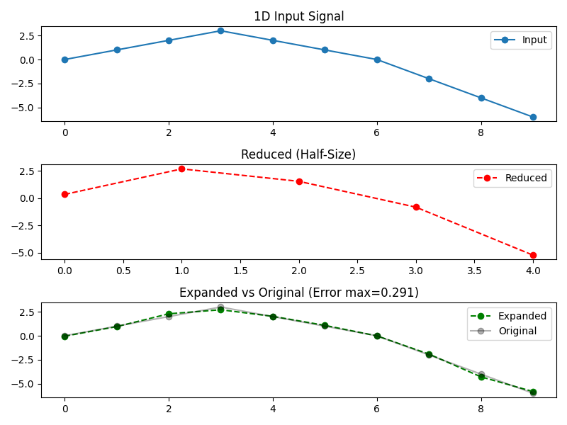
[1D Pyramid Test]
Filter: 'Centered Spline' (order=3), is_centered=True
Input   x: [ 0.  1.  2.  3.  2.  1.  0. -2. -4. -6.]
Reduced   : [ 0.34065843  2.68175207  1.54133046 -0.83042701 -5.23331582]
Expanded  : [-0.04459776  0.95501393  2.29130194  2.71324125  2.02602713  1.08397035
 -0.01051075 -1.9097665  -4.28487695 -5.81974832]
Error     : [-0.04459776 -0.04498607  0.29130194 -0.28675875  0.02602713  0.08397035
 -0.01051075  0.0902335  -0.28487695  0.18025168]

Load and Normalize a 2D Image

Here, we load an example image from an online repository. We convert it to grayscale in [0,1].

url = 'https://r0k.us/graphics/kodak/kodak/kodim07.png'
response = requests.get(url)
img = Image.open(BytesIO(response.content))

# Convert to numpy float64
image_color = np.array(img, dtype=np.float64)

# Normalize to [0,1]
image_color /= 255.0

# Convert to grayscale using standard weights
image_gray = (
    image_color[:, :, 0] * 0.2989 +
    image_color[:, :, 1] * 0.5870 +
    image_color[:, :, 2] * 0.1140
)

ny, nx = image_gray.shape
print(f"Downloaded image shape = {ny} x {nx}")

# Plot the original grayscale image
plt.figure(figsize=(6, 6))
plt.imshow(image_gray, cmap='gray', interpolation='nearest', vmin=0, vmax=1)
plt.title("Original Grayscale Image", fontsize=14)
plt.axis('off')
plt.tight_layout()
plt.show()

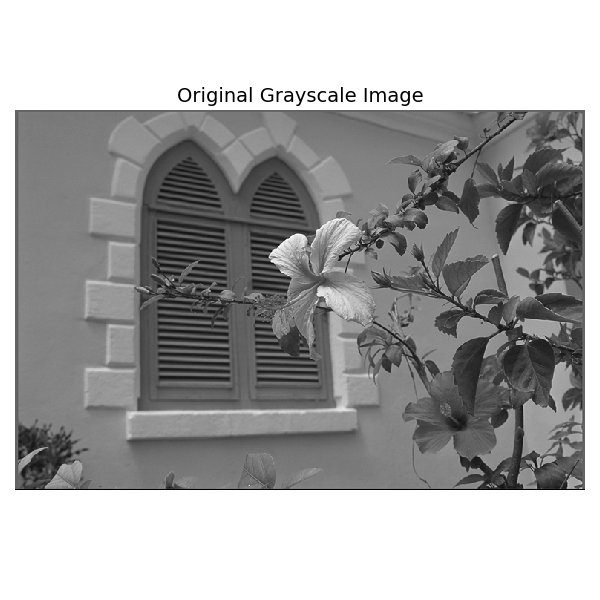
Downloaded image shape = 512 x 768

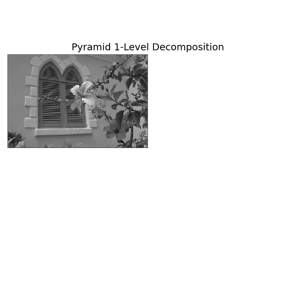
2D Pyramid Decomposition

Reduce and expand the input image using spline pyramid decomposition.

filter_name = "Spline"
order = 3
g, h, is_centered = get_pyramid_filter(filter_name, order)

reduced_2d = reduce_2d(image_gray, g, is_centered)
expanded_2d = expand_2d(reduced_2d, h, is_centered)
error_2d = expanded_2d - image_gray
max_err = np.abs(error_2d).max()

print("[2D Pyramid Test]")
print(f"Filter: '{filter_name}' (order={order}), is_centered={is_centered}")
print("Reduced shape:", reduced_2d.shape)
print("Expanded shape:", expanded_2d.shape)
print(f"Max error: {max_err}")

# Retrieve the pyramid filter parameters (using "Spline" filter with order 3)
filter_name = "Spline"
order = 3
g, h, is_centered = get_pyramid_filter(filter_name, order)

# Compute pyramid levels:
# Level 0: Original image, and each subsequent level is obtained by reducing the previous one.
num_reductions = 3
levels = []
current = image_gray  # image_gray is already loaded from previous cell.
levels.append(current)  # Level 0: Original image
for _ in range(num_reductions):
    current = reduce_2d(current, g, is_centered)
    levels.append(current)

original_shape = image_gray.shape  # (ny, nx)

[2D Pyramid Test]
Filter: 'Spline' (order=3), is_centered=False
Reduced shape: (256, 384)
Expanded shape: (512, 768)
Max error: 0.5062710854288006

1-Level Decomposition

canvas1 = np.ones(original_shape, dtype=image_gray.dtype)  # white canvas
h1, w1 = levels[1].shape
canvas1[:h1, :w1] = levels[1]  # Place the reduced image in the top-left corner

plt.figure(figsize=(6, 6))
plt.imshow(canvas1, cmap='gray', vmin=0, vmax=1, interpolation='nearest')
plt.title("Pyramid 1-Level Decomposition", fontsize=14)
plt.axis('off')
plt.tight_layout()
plt.show()

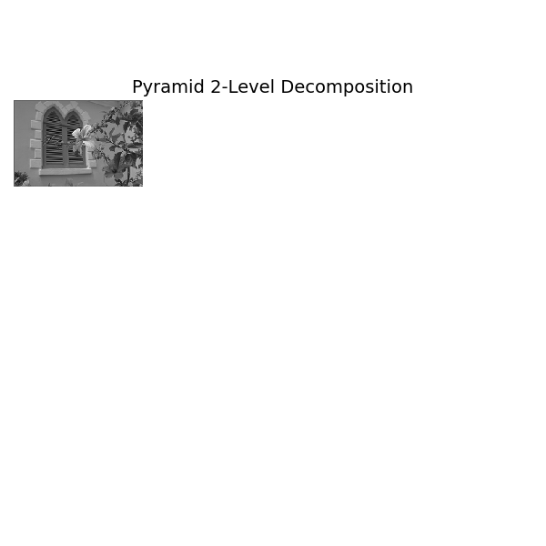
2-Level Decomposition

canvas2 = np.ones(original_shape, dtype=image_gray.dtype)  # white canvas
h2, w2 = levels[2].shape
canvas2[:h2, :w2] = levels[2]  # Place the reduced image in the top-left corner

plt.figure(figsize=(6, 6))
plt.imshow(canvas2, cmap='gray', vmin=0, vmax=1, interpolation='nearest')
plt.title("Pyramid 2-Level Decomposition", fontsize=14)
plt.axis('off')
plt.tight_layout()
plt.show()

3-Level Decomposition

canvas3 = np.ones(original_shape, dtype=image_gray.dtype)  # white canvas
h3, w3 = levels[3].shape
canvas3[:h3, :w3] = levels[3]  # Place the reduced image in the top-left corner

plt.figure(figsize=(6, 6))
plt.imshow(canvas3, cmap='gray', vmin=0, vmax=1, interpolation='nearest')
plt.title("Pyramid 3-Level Decomposition", fontsize=14)
plt.axis('off')
plt.tight_layout()
plt.show()

2D Wavelet Decomposition

We demonstrate wavelet decomposition (analysis) and reconstruction (synthesis) using 2D Haar wavelets on a grayscale image.

haar2d = HaarWavelets(scales=3)
coeffs = haar2d.analysis(image_gray)
recon_haar = haar2d.synthesis(coeffs)
err_haar = recon_haar - image_gray
max_err_haar = np.abs(err_haar).max()

print("[Wavelets 2D Haar Test]")
print(f"Max error after 3-scale decomposition: {max_err_haar}")

# Helper function for visualization
def pyramid_with_quadrant_embedding_levels(wavelet, inp, num_levels):
    """
    Perform multi-scale wavelet analysis in-place so that at each level the
    new coarse approximation is stored in the quadrant corresponding to the
    previous level's coarse region.

    Parameters
    ----------
    wavelet : AbstractWavelets instance
        A wavelet instance (e.g., HaarWavelets) with the desired number of scales.
    inp : np.ndarray
        Input 2D array (e.g., grayscale image).
    num_levels : int
        The number of decomposition levels to perform.

    Returns
    -------
    coeffs : np.ndarray
        Final coefficient array (same size as inp) with the pyramid layout.
    """
    out = np.copy(inp)
    ny, nx = out.shape[:2]

    for level in range(num_levels):
        # Process the current top-left subarray
        sub = out[:ny, :nx]
        sub_out = wavelet.analysis1(sub)
        out[:ny, :nx] = sub_out

        # Update region size for next level (halve each dimension)
        nx = max(1, nx // 2)
        ny = max(1, ny // 2)

    return out

[Wavelets 2D Haar Test]
Max error after 3-scale decomposition: 1.3322676295501878e-15

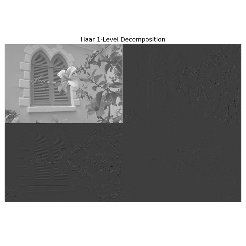
1-Level Decomposition

wavelet1 = HaarWavelets(scales=1)
coeffs1 = pyramid_with_quadrant_embedding_levels(wavelet1, image_gray, 1)

plt.figure(figsize=(8, 8))
plt.imshow(coeffs1, cmap='gray', interpolation='nearest')
plt.title("Haar 1-Level Decomposition", fontsize=14)
plt.axis('off')
plt.tight_layout()
plt.show()

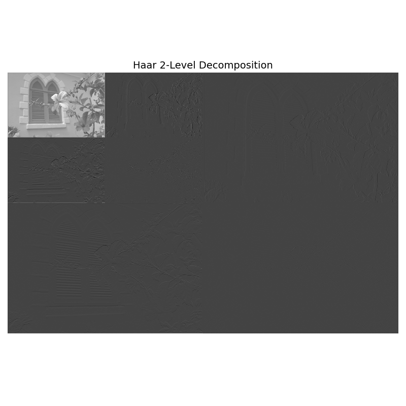
2-Level Decomposition

wavelet2 = HaarWavelets(scales=2)
coeffs2 = pyramid_with_quadrant_embedding_levels(wavelet2, image_gray, 2)

plt.figure(figsize=(8, 8))
plt.imshow(coeffs2, cmap='gray', interpolation='nearest')
plt.title("Haar 2-Level Decomposition", fontsize=14)
plt.axis('off')
plt.tight_layout()
plt.show()

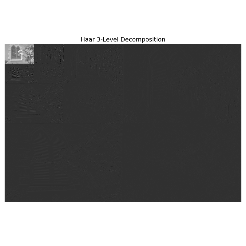
3-Level Decomposition

wavelet3 = HaarWavelets(scales=3)
coeffs3 = pyramid_with_quadrant_embedding_levels(wavelet3, image_gray, 3)

plt.figure(figsize=(8, 8))
plt.imshow(coeffs3, cmap='gray', interpolation='nearest')
plt.title("Haar 3-Level Decomposition", fontsize=14)
plt.axis('off')
plt.tight_layout()
plt.show()