Interpolate 2D Images

Interpolate 2D images with standard interpolation, least-squares, and oblique projection. Compare them to SciPy zoom. We compute SNR and MSE only on a central region to exclude boundary artifacts. A summary of the cost/benefit tradeoff of the three methods is provided at the bottom of this page.

You can download this example at the tab at right (Python script or Jupyter notebook.

Required Libraries

We import the required libraries, including NumPy for numerical computations, Matplotlib for plotting, and the custom resize function from the splineops package.

import numpy as np
import matplotlib.pyplot as plt
import requests
from io import BytesIO
from PIL import Image
from scipy.ndimage import zoom  # For SciPy's zoom comparison
from splineops.resize.resize import resize  # Unified resize function
import time

Helper Functions

We define

• a utility to crop out ~20% borders around the image;

• SNR and MSE on that central cropped area;

• resizing functions.

def crop_to_central_region(image, border_fraction):
    """
    Return a central sub-region of 'image', skipping 'border_fraction'
    of the width/height on all sides.
    """
    H, W = image.shape
    top = int(H * border_fraction)
    bottom = int(H * (1 - border_fraction))
    left = int(W * border_fraction)
    right = int(W * (1 - border_fraction))
    # Guard against degenerate cases
    top = max(top, 0)
    left = max(left, 0)
    bottom = min(bottom, H)
    right = min(right, W)
    return image[top:bottom, left:right]


def compute_snr_and_mse_cropped(original, processed, border_fraction):
    """
    Compute SNR and MSE on the 'central' cropped area, ignoring border_fraction
    of the image on each side.
    """
    # Crop both images consistently
    orig_cropped = crop_to_central_region(original, border_fraction)
    proc_cropped = crop_to_central_region(processed, border_fraction)

    # Now compute SNR/MSE on that region
    signal_power = np.mean(orig_cropped**2)
    noise_power = np.mean((orig_cropped - proc_cropped)**2)
    mse_val = noise_power

    if noise_power <= 1e-30:  # near-zero difference
        snr_val = float('inf')
    else:
        snr_val = 10 * np.log10(signal_power / noise_power)

    return snr_val, mse_val


def resize_with_scipy_zoom(input_image, zoom_factors, degree, border_fraction):
    """
    Resize using SciPy's zoom, then resize back and compute SNR/MSE
    *only on a central region* to avoid boundary artifacts.
    """
    start_time = time.perf_counter()
    resized_image = zoom(input_image, zoom_factors, order=degree)
    time_elapsed = time.perf_counter() - start_time

    reverse_zoom_factors = 1.0 / np.array(zoom_factors)
    recovered_image = zoom(resized_image, reverse_zoom_factors, order=degree)

    # Compute SNR/MSE on central region
    snr, mse = compute_snr_and_mse_cropped(input_image, recovered_image, border_fraction)

    return resized_image, recovered_image, snr, mse, time_elapsed


def resize_and_compute_metrics(input_image, method, degree, zoom_factors, border_fraction):
    """
    Resize a 2D image using the specified method, then resize back
    to original size and compute SNR, MSE, and timing *only on a central region*.
    """
    if np.isscalar(zoom_factors):
        zoom_factors = (zoom_factors, zoom_factors)

    if method == "scipy":
        return resize_with_scipy_zoom(
            input_image, zoom_factors, degree, border_fraction
        )
    else:
        start_time = time.perf_counter()
        resized_image = resize(
            data=input_image,
            zoom_factors=zoom_factors,
            degree=degree,
            method=method
        )
        time_elapsed = time.perf_counter() - start_time

        # Resize back to original shape:
        original_shape = input_image.shape
        recovered_image = resize(
            data=resized_image,
            output_size=original_shape,
            degree=degree,
            method=method
        )

        # Compute SNR/MSE on central region
        snr, mse = compute_snr_and_mse_cropped(input_image, recovered_image, border_fraction)

        return resized_image, recovered_image, snr, mse, time_elapsed

Plot Helpers

We define three plotting helpers.

1. plot_resized_image(): Show the resized 2D image

2. plot_recovered_image(): Show the image after resizing back

3. plot_difference_image(): Show the difference (original - recovered)

def plot_resized_image(original, resized, method, zoom_factors, time_elapsed):
    """
    Display the resized 2D image. If any zoom factor < 1, we place
    the resized image on a white canvas matching the original shape.
    """
    zoom_out = any(zf < 1.0 for zf in zoom_factors)

    # Convert images to 0..255 for visualization
    def to_uint8(arr):
        arr_min, arr_max = arr.min(), arr.max()
        if arr_max > arr_min:
            arr_scaled = (arr - arr_min) / (arr_max - arr_min)
        else:
            arr_scaled = arr * 0.0
        return (arr_scaled * 255).astype(np.uint8)

    orig_8 = to_uint8(original)
    resized_8 = to_uint8(resized)

    if zoom_out:
        canvas_8 = np.full_like(orig_8, 255, dtype=np.uint8)  # white canvas
        rh, rw = resized_8.shape
        canvas_8[:rh, :rw] = resized_8
        resized_display = canvas_8
    else:
        resized_display = resized_8

    plt.figure(figsize=(5, 5))
    plt.imshow(resized_display, cmap='gray', aspect='equal')
    plt.title(
        f"{method.capitalize()} Resized\n"
        f"Zoom: {zoom_factors}, Time: {time_elapsed:.4f}s"
    )
    plt.axis('off')
    plt.show()

def plot_recovered_image(recovered):
    """
    Display the recovered image after resizing back to the original shape.
    """
    plt.figure(figsize=(6, 5))
    plt.imshow(recovered, cmap='gray', aspect='equal')
    plt.title("Recovered Image")
    plt.axis('off')
    plt.show()

from mpl_toolkits.axes_grid1 import make_axes_locatable

def plot_difference_image(original, recovered, snr, mse):
    """
    Display the difference (original - recovered) with a colorbar
    that fits the image height and preserves aspect ratio.

    The difference is shown in the *original numeric range*, not uint8,
    so the colorbar reflects the actual difference scale.

    Color scale is fixed to [-0.8, +0.8] for consistency across plots.
    """
    difference = original - recovered
    h, w = difference.shape  # shape of the difference image

    # Compute aspect ratio (height / width).
    aspect_ratio = h / float(w)

    # Choose a reference figure width and derive the figure height
    # to preserve the aspect ratio. Adjust fig_width as needed.
    fig_width = 6.0
    fig_height = fig_width * aspect_ratio

    fig, ax = plt.subplots(figsize=(fig_width, fig_height))

    im = ax.imshow(
        difference,
        cmap='bwr',
        aspect='equal',  # ensure each pixel is square
        vmin=-0.8,
        vmax=0.8
    )

    ax.set_title(f"Difference\nSNR: {snr:.2f} dB, MSE: {mse:.2e}")
    ax.axis('off')

    # Use make_axes_locatable to create a colorbar axis matching the image height
    divider = make_axes_locatable(ax)
    cax = divider.append_axes("right", size="5%", pad=0.05)  # colorbar is 5% width, 0.05 pad

    cb = plt.colorbar(im, cax=cax)
    cb.set_label('Difference (units)')

    plt.tight_layout()
    plt.show()

Load and Normalize an Image

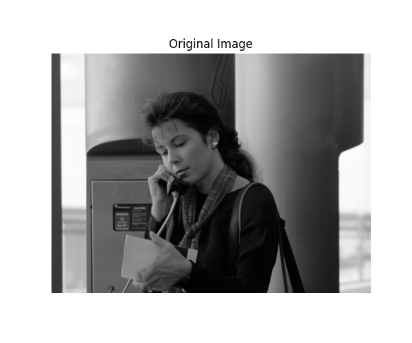
Here, we load an example image from an online repository. We convert it to grayscale in [0, 1].

url = 'https://people.math.sc.edu/Burkardt/data/tif/columns.tif'
response = requests.get(url)
img = Image.open(BytesIO(response.content))
data = np.array(img, dtype=np.float64)

# Convert to [0..1]
input_image_normalized = data / 255.0

# Convert to grayscale via simple weighting
input_image_normalized = (
    input_image_normalized[:, :, 0] * 0.2989 +  # Red channel
    input_image_normalized[:, :, 1] * 0.5870 +  # Green channel
    input_image_normalized[:, :, 2] * 0.1140    # Blue channel
)

degree = 3
zoom_factors_2d = (0.25, 0.25)
border_fraction = 0.3

# We plot the original grayscale image.

plt.figure(figsize=(6, 5))
plt.imshow(input_image_normalized, cmap='gray', aspect='equal')
plt.title("Original Image")
plt.axis("off")
plt.show()

SciPy Interpolation

For comparison purposes, we also use the SciPy zoom method for resizing.

(
    resized_2d_scipy,
    recovered_2d_scipy,
    snr_2d_scipy,
    mse_2d_scipy,
    time_2d_scipy
) = resize_and_compute_metrics(
    input_image_normalized,
    method="scipy",
    degree=degree,
    zoom_factors=zoom_factors_2d,
    border_fraction=border_fraction
)

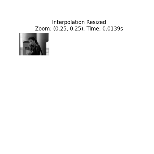
Resized Image

We plot the resized image with SciPy interpolation.

plot_resized_image(
    original=input_image_normalized,
    resized=resized_2d_scipy,
    method="scipy",
    zoom_factors=zoom_factors_2d,
    time_elapsed=time_2d_scipy
)

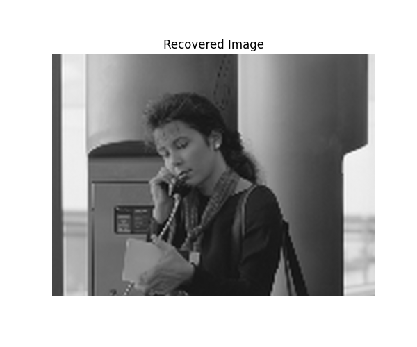
Recovered Image

We plot the recovered image after a reversing of the zoom factors.

plot_recovered_image(recovered_2d_scipy)

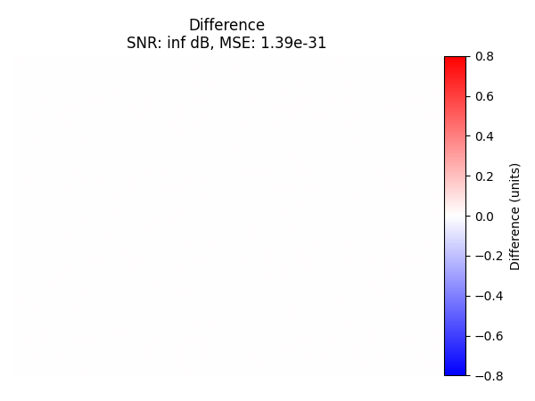
Difference Image

Display the difference image (original - recovered) with colorbar.

plot_difference_image(
    original=input_image_normalized,
    recovered=recovered_2d_scipy,
    snr=snr_2d_scipy,
    mse=mse_2d_scipy
)

Trivial Interpolation

We use our standard interpolation method.

(
    resized_2d_interp,
    recovered_2d_interp,
    snr_2d_interp,
    mse_2d_interp,
    time_2d_interp
) = resize_and_compute_metrics(
    input_image_normalized,
    method="interpolation",
    degree=degree,
    zoom_factors=zoom_factors_2d,
    border_fraction=border_fraction
)

Resized Image

We plot the resized image with standard interpolation.

plot_resized_image(
    original=input_image_normalized,
    resized=resized_2d_interp,
    method="interpolation",
    zoom_factors=zoom_factors_2d,
    time_elapsed=time_2d_interp
)

Recovered Image

We plot the recovered image after a reversing of the zoom factors.

plot_recovered_image(recovered_2d_interp)

Difference image

Display the difference image (original - recovered) with colorbar.

plot_difference_image(
    original=input_image_normalized,
    recovered=recovered_2d_interp,
    snr=snr_2d_interp,
    mse=mse_2d_interp
)

Difference with SciPy

Now we compute the difference between the recovered image from the trivial interpolation and the SciPy interpolation. We also compute SNR and MSE on the central region and display them. Because they are nearly identical, we conclude that the two interpolation methods produce the same results.

snr_scipy_vs_interp, mse_scipy_vs_interp = compute_snr_and_mse_cropped(
    recovered_2d_scipy, recovered_2d_interp, border_fraction
)

plot_difference_image(
    original=recovered_2d_scipy,
    recovered=recovered_2d_interp,
    snr=snr_scipy_vs_interp,
    mse=mse_scipy_vs_interp
)

Alternative with TensorSpline

As an alternative, we can replicate the same interpolation manually using the TensorSpline class, which underpins the resize() function behind the scene.

from splineops.interpolate.tensorspline import TensorSpline

# 1) Build uniform coordinate arrays that match the shape of 'input_image_normalized'

height, width = input_image_normalized.shape
x_coords = np.linspace(0, height - 1, height)
y_coords = np.linspace(0, width - 1, width)
coordinates_2d = (x_coords, y_coords)

# 2) For "cubic interpolation", pick "bspline3".
#    For boundary handling, we can pick "mirror", "zero", etc.

ts = TensorSpline(
    data=input_image_normalized,
    coordinates=coordinates_2d,
    bases="bspline3",  # cubic B-splines
    modes="mirror"     # handles boundaries with mirroring
)

# 3) Define new coordinate grids for the "zoomed" shape.

zoomed_height = int(height * zoom_factors_2d[0])
zoomed_width = int(width * zoom_factors_2d[1])

x_coords_zoomed = np.linspace(0, height - 1, zoomed_height)
y_coords_zoomed = np.linspace(0, width - 1, zoomed_width)
coords_zoomed_2d = (x_coords_zoomed, y_coords_zoomed)

# Evaluate (forward pass): zoom in or out

resized_direct_ts = ts(coordinates=coords_zoomed_2d)

# 4) Define coordinate grids for returning to the original shape
x_coords_orig = np.linspace(0, height - 1, height)
y_coords_orig = np.linspace(0, width - 1, width)
coords_orig_2d = (x_coords_orig, y_coords_orig)

# Evaluate (backward pass): from zoomed shape back to original

ts_zoomed = TensorSpline(
    data=resized_direct_ts,
    coordinates=coords_zoomed_2d,
    bases="bspline3",
    modes="mirror"
)
recovered_direct_ts = ts_zoomed(coordinates=coords_orig_2d)

# Now, resized_direct_ts / recovered_direct_ts should be very similar
# to 'resized_2d_interp' / 'recovered_2d_interp' from the high-level "resize()" approach.
# Let's compute MSE to confirm:

mse_forward = np.mean((resized_direct_ts - resized_2d_interp) ** 2)
mse_backward = np.mean((recovered_direct_ts - recovered_2d_interp) ** 2)
print(f"MSE (TensorSpline vs. resize()) resized:  {mse_forward:.6e}")
print(f"MSE (TensorSpline vs. resize()) recovered: {mse_backward:.6e}")

MSE (TensorSpline vs. resize()) resized:  0.000000e+00
MSE (TensorSpline vs. resize()) recovered: 1.133506e-30

Least-Squares Projection

We use the least-squares projection method.

(
    resized_2d_ls,
    recovered_2d_ls,
    snr_2d_ls,
    mse_2d_ls,
    time_2d_ls
) = resize_and_compute_metrics(
    input_image_normalized,
    method="least-squares",
    degree=degree,
    zoom_factors=zoom_factors_2d,
    border_fraction=border_fraction
)

Resized Image

We plot the resized image with least-squares projection method.

plot_resized_image(
    original=input_image_normalized,
    resized=resized_2d_ls,
    method="least-squares",
    zoom_factors=zoom_factors_2d,
    time_elapsed=time_2d_ls
)

Recovered Image

We plot the recovered image after reversing zoom factors.

plot_recovered_image(recovered_2d_ls)

Difference Image

Display the difference image (original - recovered) with colorbar.

plot_difference_image(
    original=input_image_normalized,
    recovered=recovered_2d_ls,
    snr=snr_2d_ls,
    mse=mse_2d_ls
)

Oblique Projection

We use the oblique-projection method.

(
    resized_2d_ob,
    recovered_2d_ob,
    snr_2d_ob,
    mse_2d_ob,
    time_2d_ob
) = resize_and_compute_metrics(
    input_image_normalized,
    method="oblique",
    degree=degree,
    zoom_factors=zoom_factors_2d,
    border_fraction=border_fraction
)

Resized Image

We plot the resized image with the oblique-projection method.

plot_resized_image(
    original=input_image_normalized,
    resized=resized_2d_ob,
    method="oblique",
    zoom_factors=zoom_factors_2d,
    time_elapsed=time_2d_ob
)

Recovered Image

We plot the recovered image after a reversing of the zoom factors.

plot_recovered_image(recovered_2d_ob)

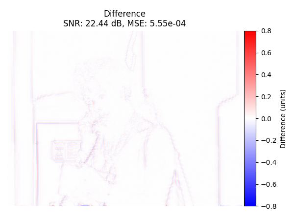
Difference Image

Display the difference image (original - recovered) with colorbar.

plot_difference_image(
    original=input_image_normalized,
    recovered=recovered_2d_ob,
    snr=snr_2d_ob,
    mse=mse_2d_ob
)

Comparison

We compare the performance of the different methods being analyzed.

Comparison Table

We print the SNR, MSE, and timing data for each method.

methods = [
    ("SciPy Interpolation", snr_2d_scipy, mse_2d_scipy, time_2d_scipy),
    ("Trivial Interpolation", snr_2d_interp, mse_2d_interp, time_2d_interp),
    ("Least-Squares Projection", snr_2d_ls, mse_2d_ls, time_2d_ls),
    ("Oblique Projection", snr_2d_ob, mse_2d_ob, time_2d_ob),
]

# Print the table header using the same widths as we'll use for data
header_line = f"{'Method':<25} {'SNR (dB)':>10} {'MSE':>16} {'Time (s)':>12}"
print(header_line)
print("-" * len(header_line))  # or manually set a dash length, e.g. 67

# Now print each row with the matching format
for method_name, snr_val, mse_val, time_val in methods:
    row_line = f"{method_name:<25} {snr_val:>10.2f} {mse_val:>16.2e} {time_val:>12.4f}"
    print(row_line)

Method                      SNR (dB)              MSE     Time (s)
------------------------------------------------------------------
SciPy Interpolation            20.62         8.45e-04       0.0074
Trivial Interpolation          20.62         8.45e-04       0.0139
Least-Squares Projection       22.52         5.45e-04       1.1896
Oblique Projection             22.44         5.55e-04       0.9304

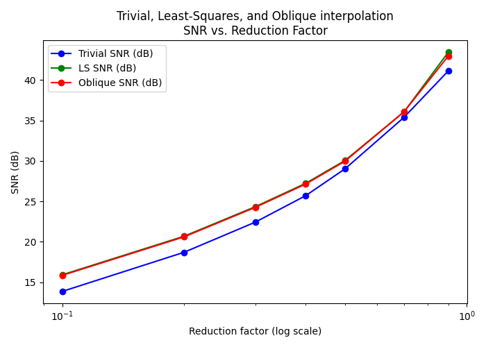
Comparison Plot

Here, we compare how standard interpolation, least-squares, and oblique projection perform (in terms of SNR) across multiple zoom factors in [0.05, 0.9]. For each method at each zoom factor, we compute the SNR between the recovered image and the original, and plot the results on a single y-axis. Note that we don’t compare with Scipy interpolation as it virtually gives the same values as the trivial interpolation.

zoom_values = np.array([0.1, 0.2, 0.3, 0.4, 0.5, 0.7, 0.9])

snr_scipy_list = []
snr_ls_list = []
snr_ob_list = []

for z in zoom_values:
    # Interpolation
    _, recovered_scipy, snr_scipy_z, _, _ = resize_and_compute_metrics(
        input_image_normalized,
        method="interpolation",
        degree=degree,
        zoom_factors=z,
        border_fraction=border_fraction
    )
    snr_scipy_list.append(snr_scipy_z)

    # Least-Squares
    _, recovered_ls, snr_ls_z, _, _ = resize_and_compute_metrics(
        input_image_normalized,
        method="least-squares",
        degree=degree,
        zoom_factors=z,
        border_fraction=border_fraction
    )
    snr_ls_list.append(snr_ls_z)

    # Oblique
    _, recovered_ob, snr_ob_z, _, _ = resize_and_compute_metrics(
        input_image_normalized,
        method="oblique",
        degree=degree,
        zoom_factors=z,
        border_fraction=border_fraction
    )
    snr_ob_list.append(snr_ob_z)

# Now we plot SNR in the same figure
fig, ax1 = plt.subplots(figsize=(7, 5))

# Plot SNR (dB)
p1 = ax1.plot(zoom_values, snr_scipy_list, 'bo-', label='Trivial SNR (dB)')
p2 = ax1.plot(zoom_values, snr_ls_list,    'go-', label='LS SNR (dB)')
p3 = ax1.plot(zoom_values, snr_ob_list,    'ro-', label='Oblique SNR (dB)')

# Set the reduction factor axis to log scale
ax1.set_xscale('log')
ax1.set_xlabel('Reduction factor (log scale)')
ax1.set_ylabel('SNR (dB)')

ax1.set_title('Trivial, Least-Squares, and Oblique interpolation\nSNR vs. Reduction Factor')

ax1.legend(loc='best')

plt.tight_layout()
plt.show()