Interpolate 1D Samples#
Interpolate 1D samples with standard interpolation.
Assume that a user-provided 1D list of samples \(f[k]\) has been obtained by sampling a spline on a unit grid.
From the samples, recover the continuously defined spline \(f(x)\).
Resample \(f(x)\) to get \(g[k] = f(\lambda k)\), with \(|\lambda| > 1\).
Create a new spline \(g(x)\) from the samples \(g[k]\).
We define \(h(x) = g(x / \lambda)\).
Compute the mean squared error (MSE) between \(f\) and \(h\).
You can download this example at the tab at right (Python script or Jupyter notebook.
Required Libraries#
We import the required libraries, including numpy for numerical computations, Matplotlib for the plots, and the splineops package.
import numpy as np
import matplotlib.pyplot as plt
from matplotlib.gridspec import GridSpec
from splineops.interpolate.tensorspline import TensorSpline

plt.rcParams.update({
    "font.size": 14,     # Base font size
    "axes.titlesize": 18,  # Title font size
    "axes.labelsize": 16,  # Label font size
    "xtick.labelsize": 14,
    "ytick.labelsize": 14
})
Initial 1D Samples#
We generate 1D samples and treat them as discrete signal points.
Let \(\mathbf{f} = (f[0], f[1], f[2], \dots, f[K-1])\) be a 1D array of data.
These are the input samples that we are going to interpolate.
number_of_samples = 27

f_support = np.arange(number_of_samples)
f_support_length = len(f_support) # It's equal to number_of_samples

f_samples = np.array([
    -0.657391, -0.641319, -0.613081, -0.518523, -0.453829, -0.385138,
    -0.270688, -0.179849, -0.11805, -0.0243016, 0.0130667, 0.0355389,
    0.0901577, 0.219599, 0.374669, 0.384896, 0.301386, 0.128646,
    -0.00811776, 0.0153119, 0.106126, 0.21688, 0.347629, 0.419532,
    0.50695, 0.544767, 0.555373
])

plt.figure(figsize=(10, 4))
plt.title("f[k] samples")
plt.stem(f_support, f_samples, basefmt=" ")
# Add a black horizontal line at y=0:
plt.axhline(
    y=0,
    color="black",
    linewidth=1,
    zorder=0
)
plt.xlabel("k")
plt.ylabel("f[k]")
plt.grid(True)
plt.tight_layout()
plt.show()
![f[k] samples](../_images/sphx_glr_002_interpolate_1D_samples_001.png)
Interpolate the Samples with a Spline#
We interpolate the 1D samples with a spline to obtain the continuously defined function
where
the B-spline of degree \(n\) is \(\beta^n\);
the spline coefficients \(c[k]\) are determined from the input samples, such that \(f(k) = f[k]\).
Let us now plot \(f\).
# Plot points
plot_points_per_unit = 12

# Interpolated signal
base = "bspline3"
mode = "mirror"
TensorSpline#
Here is one way to perform the standard interpolation.
f = TensorSpline(data=f_samples, coordinates=f_support, bases=base, modes=mode)

f_coords = np.array([q / plot_points_per_unit
                        for q in range(plot_points_per_unit * f_support_length)])

# Syntax hint: pass (plot_coords,) not plot_coords
f_data = f(coordinates=(f_coords,), grid=False)
Resize Method#
The resize method with standard interpolation yields the same result.
from splineops.resize.resize import resize

# We'll produce the same number of output samples as in f_coords
desired_length = plot_points_per_unit * f_support_length

# IMPORTANT: We explicitly define a coordinate array from 0..(f_support_length - 1)
# with `desired_length` points. This matches the domain and size that the `resize`
# function will produce below, ensuring the two outputs are sampled at the exact
# same x-positions, and thus comparable point-by-point.
f_coords_resize = np.linspace(0, f_support_length - 1, desired_length)

f_data_resize = resize(
    data=f_samples,             # 1D input
    output_size=(desired_length,),
    degree=3,                   # matches "bspline3"
    method="interpolation"      # ensures TensorSpline standard interpolation, not least-squares or oblique
)

# Ensure both arrays have identical shapes
f_data_spline = f(coordinates=(f_coords_resize,), grid=False)
assert f_data_spline.shape == f_data_resize.shape, "Arrays must match in shape."
mse_diff = np.mean((f_data_spline - f_data_resize)**2)
print(f"MSE between TensorSpline result and resize result = {mse_diff:.6e}")
MSE between TensorSpline result and resize result = 0.000000e+00
Plot of the Spline f#
plt.figure(figsize=(10, 4))
plt.title("f[k] samples with interpolated f spline")
plt.stem(f_support, f_samples, basefmt=" ", label="f[k] samples")
# Add a black horizontal line at y=0:
plt.axhline(
    y=0,
    color="black",
    linewidth=1,
    zorder=0 # draw behind other plot elements
)
plt.plot(f_coords_resize, f_data_resize, color="green", linewidth=2, label="f spline")
plt.xlabel("k")
plt.ylabel("f")
plt.legend()
plt.grid(True)
plt.tight_layout()
plt.show()
![f[k] samples with interpolated f spline](../_images/sphx_glr_002_interpolate_1D_samples_002.png)
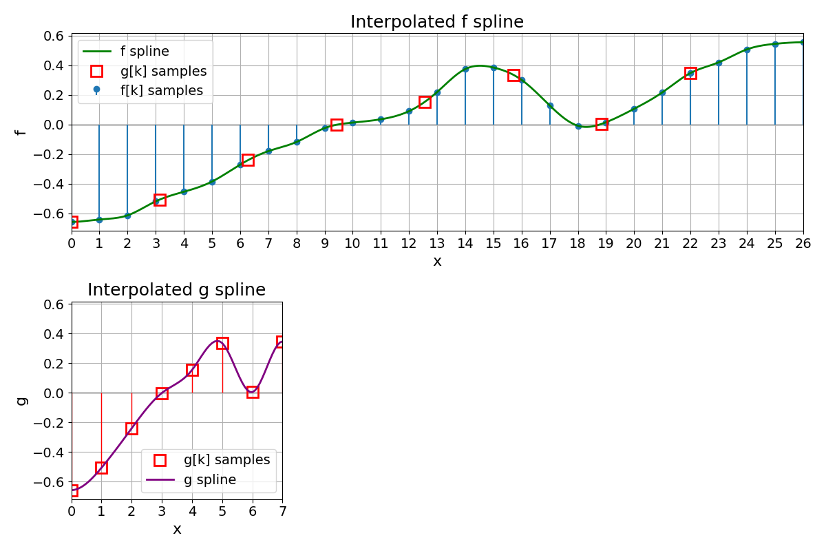
Coarsening of f#
We define \(\lambda\) with \(|\lambda| > 1\) and sample \(f(x)\) at \(x = \lambda k\) as
These points \(g[k]\) form a new discrete set, which we then treat as a separate signal to build another spline \(g\).
val_lambda = np.pi

g_support_length = round(f_support_length // val_lambda)
g_support = np.arange(g_support_length)
f_resampled_coords = np.array([q * val_lambda for q in range(g_support_length)])
g_samples = f(coordinates=(f_resampled_coords,), grid=False)
g = TensorSpline(data=g_samples, coordinates=g_support, bases=base, modes=mode)

g_coords = np.array([q/plot_points_per_unit
                     for q in range(plot_points_per_unit * len(g_support))])
g_data = g(coordinates=(g_coords,), grid=False)

fig = plt.figure(figsize=(12, 8))

gs = GridSpec(
    nrows=2,
    ncols=2,
    # Match widths: first column = g_support_length, second column = leftover
    width_ratios=[g_support_length, f_support_length - g_support_length],
    height_ratios=[1, 1]
)

# Top row: entire row (two columns combined)
ax_top = fig.add_subplot(gs[0, :])

# Bottom row: left side for g, right side blank
ax_bottom_left = fig.add_subplot(gs[1, 0])
ax_bottom_right = fig.add_subplot(gs[1, 1])
ax_bottom_right.axis("off")  # leave right side blank

# 1) TOP ROW: f[k] + f spline + discrete g[k]
ax_top.set_title("Interpolated f spline")

# Plot discrete f[k] as stems
ax_top.stem(f_support, f_samples, basefmt=" ", label="f[k] samples")

# Plot spline f(x)
ax_top.plot(f_coords, f_data, color="green", linewidth=2, label="f spline")

# Overplot discrete g[k] as unfilled red squares at x = k * val_lambda
x_g = np.arange(g_support_length) * val_lambda
ax_top.plot(
    x_g,
    g_samples,
    "rs",              # red squares
    mfc='none',        # unfilled
    markersize=12,
    markeredgewidth=2,
    label="g[k] samples"
)

# Horizontal line at 0 for reference
ax_top.axhline(0, color='black', linewidth=1, zorder=0)

# Make sure the top axis goes from 0..(f_support_length-1)
ax_top.set_xlim(0, f_support_length - 1)
ax_top.set_xticks(np.arange(0, f_support_length, 1))
ax_top.set_xlabel("x")
ax_top.set_ylabel("f")
ax_top.grid(True)
ax_top.legend()

# 2) BOTTOM LEFT: discrete g[k] + g spline
ax_bottom_left.set_title("Interpolated g spline")

# Plot discrete g[k] with red vertical lines and unfilled red squares
ax_bottom_left.vlines(
    x=g_support,
    ymin=0,
    ymax=g_samples,
    color='red',
    linestyle='-',
    linewidth=1
)
ax_bottom_left.plot(
    g_support,
    g_samples,
    "rs",              # red squares
    mfc='none',        # unfilled
    markersize=12,
    markeredgewidth=2,
    label="g[k] samples"
)

# Plot g spline in purple over the same domain
ax_bottom_left.plot(
    g_coords,
    g_data,
    color="purple",
    linewidth=2,
    label="g spline"
)

# Horizontal line at 0
ax_bottom_left.axhline(0, color='black', linewidth=1, zorder=0)

ax_bottom_left.set_xlim(0, g_support_length - 1)
ax_bottom_left.set_xticks(np.arange(0, g_support_length, 1))
ax_bottom_left.set_xlabel("x")
ax_bottom_left.set_ylabel("g")
ax_bottom_left.grid(True)
ax_bottom_left.legend()

# Match vertical scale with the top axis
ax_bottom_left.set_ylim(ax_top.get_ylim())

fig.tight_layout()
plt.show()
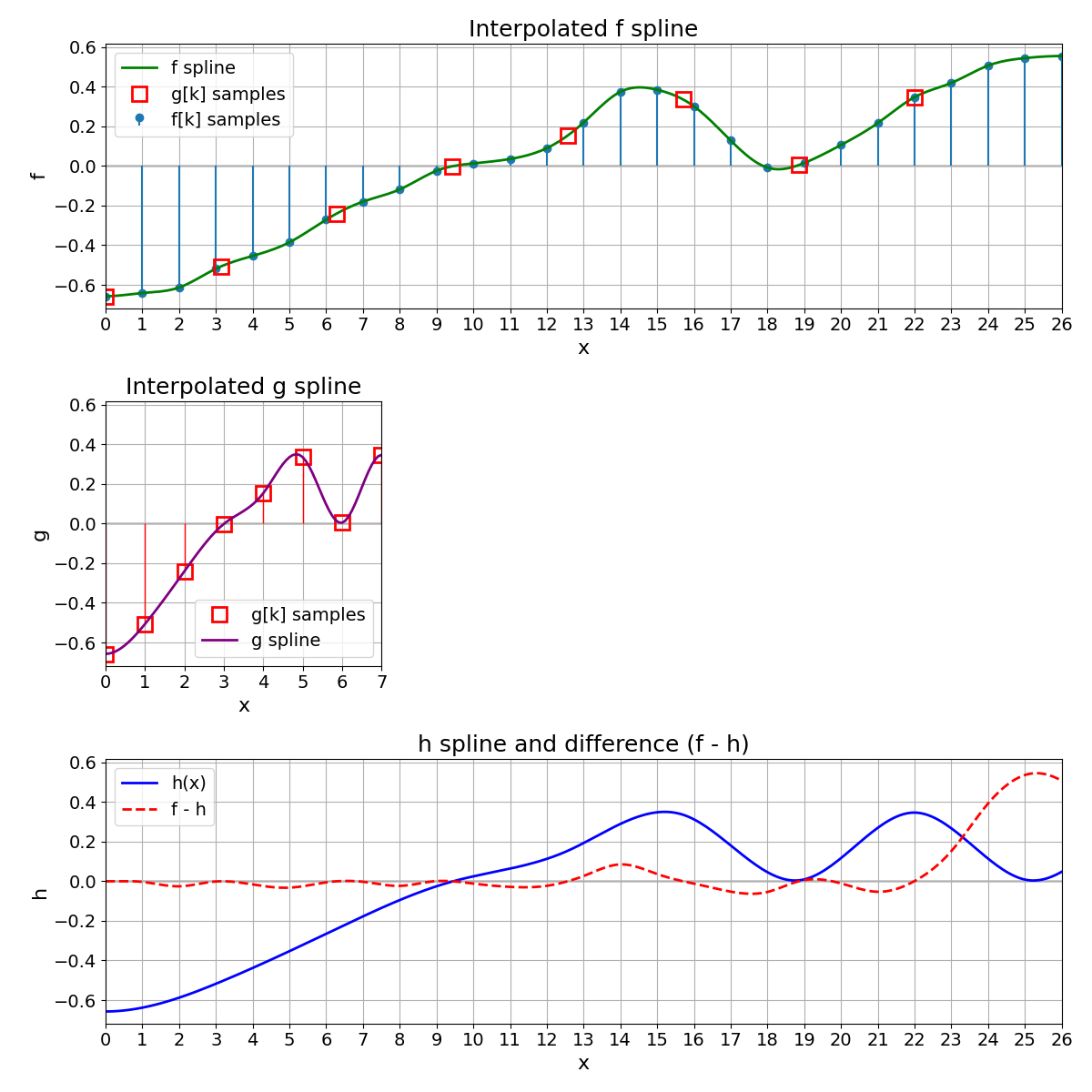
Expand g to Obtain h#
To compare \(g\) on the same domain as \(f\), we expand \(g\) by defining a new function \(h\) as
where \(g\) is the continuously defined spline built from the discrete points \(g[k]\). Hence, \(h\) and \(f\) have the same support and can be directly compared (e.g., by computing an MSE).
fig2 = plt.figure(figsize=(12, 12))

gs2 = GridSpec(
    nrows=3,
    ncols=2,
    width_ratios=[g_support_length, f_support_length - g_support_length],
    height_ratios=[1, 1, 1]  # three equal rows
)

# TOP ROW: f + f spline + discrete g[k]
ax_top = fig2.add_subplot(gs2[0, :])  # spans both columns
ax_top.set_title("Interpolated f spline")

# Replot discrete f[k] as stems
ax_top.stem(f_support, f_samples, basefmt=" ", label="f[k] samples")

# Replot f spline
ax_top.plot(f_coords, f_data, color="green", linewidth=2, label="f spline")

# Overplot discrete g[k] in red squares at x = k*val_lambda
x_g = np.arange(g_support_length) * val_lambda
ax_top.plot(
    x_g, g_samples,
    "rs", mfc='none', markersize=12, markeredgewidth=2,
    label="g[k] samples"
)

# Horizontal line at 0
ax_top.axhline(0, color="black", linewidth=1, zorder=0)

ax_top.set_xlim(0, f_support_length - 1)
ax_top.set_xticks(np.arange(0, f_support_length, 1))
ax_top.set_xlabel("x")
ax_top.set_ylabel("f")
ax_top.legend()
ax_top.grid(True)

# MIDDLE ROW: discrete g + g spline
ax_mid_left = fig2.add_subplot(gs2[1, 0])  # left cell
ax_mid_right = fig2.add_subplot(gs2[1, 1]) # right cell
ax_mid_right.axis("off")                  # keep it blank

ax_mid_left.set_title("Interpolated g spline")

# Plot discrete g[k] with red stems, unfilled squares
ax_mid_left.vlines(
    x=g_support,
    ymin=0,
    ymax=g_samples,
    color='red',
    linestyle='-',
    linewidth=1
)
ax_mid_left.plot(
    g_support,
    g_samples,
    "rs", mfc='none', markersize=12, markeredgewidth=2,
    label="g[k] samples"
)

# Plot g spline
ax_mid_left.plot(
    g_coords, g_data,
    color="purple", linewidth=2,
    label="g spline"
)

ax_mid_left.axhline(0, color='black', linewidth=1, zorder=0)
ax_mid_left.set_xlim(0, g_support_length - 1)
ax_mid_left.set_xticks(np.arange(0, g_support_length, 1))
ax_mid_left.set_xlabel("x")
ax_mid_left.set_ylabel("g")
ax_mid_left.legend()
ax_mid_left.grid(True)

# Match y-limits with top row:
ax_mid_left.set_ylim(ax_top.get_ylim())

# BOTTOM ROW: expanded h(x) = g(x / λ)
ax_bottom = fig2.add_subplot(gs2[2, :])  # spans both columns
ax_bottom.set_title("h spline and difference (f - h)")

# We'll sample h over 0..(f_support_length-1)
h_coords = f_coords
# Evaluate h(x) = g(x/val_lambda)
h_data = g(coordinates=(h_coords / val_lambda,), grid=False)

# Also evaluate f at the same coords, so we can show the difference
f_data_for_diff = f(coordinates=(h_coords,), grid=False)
diff_data = f_data_for_diff - h_data

# Plot h in blue
ax_bottom.plot(h_coords, h_data, color="blue", linewidth=2, label="h(x)")

# Plot difference f - h in red, dashed
ax_bottom.plot(h_coords, diff_data, color="red", linestyle="--", linewidth=2, label="f - h")

ax_bottom.axhline(0, color='black', linewidth=1, zorder=0)

# The domain is the same as f
ax_bottom.set_xlim(0, f_support_length - 1)
ax_bottom.set_xticks(np.arange(0, f_support_length, 1))
ax_bottom.set_xlabel("x")
ax_bottom.set_ylabel("h")
ax_bottom.grid(True)
ax_bottom.legend()

# Match y axis with top row
ax_bottom.set_ylim(ax_top.get_ylim())

fig2.tight_layout()
plt.show()
MSE Between f and h#
We compute the MSE between \(h(x)\) and \(f(x)\) as
Riemann Approximation
To estimate this integral, we discretize the interval \([a,b]\) into \(K\) points. At each point \(x_k\), we evaluate \((f(x_k) - h(x_k))^2\) and multiply by the width \(\Delta x\). Summing across all points produces the approximation
The normalization by \((b-a)\) yields the MSE.
# 1) Define a midpoint sampling domain for [a, b]
N = 1000
padding_fraction = 0.2 # We avoid artifacts near the edges by excluding part of the domain from each side
a = (f_support_length - 1) * padding_fraction
b = (f_support_length - 1) * (1 - padding_fraction)
dx = (b - a) / N
mid_x = np.linspace(a + dx/2, b - dx/2, N)  # midpoints

# 2) Evaluate f(x) and h(x) at those midpoints
f_mid = f(coordinates=(mid_x,), grid=False)
h_mid = g(coordinates=(mid_x / val_lambda,), grid=False)

# 3) Compute the midpoint Riemann sum for ∫(f(x)-h(x))^2 dx
squared_diff = (f_mid - h_mid) ** 2
integral_value = np.sum(squared_diff) * dx

# 4) Divide by (b - a) to get the MSE
mse_midpoint = integral_value / (b - a)
print(f"MSE between f and h = {mse_midpoint:.6e}")
MSE between f and h = 1.152514e-03
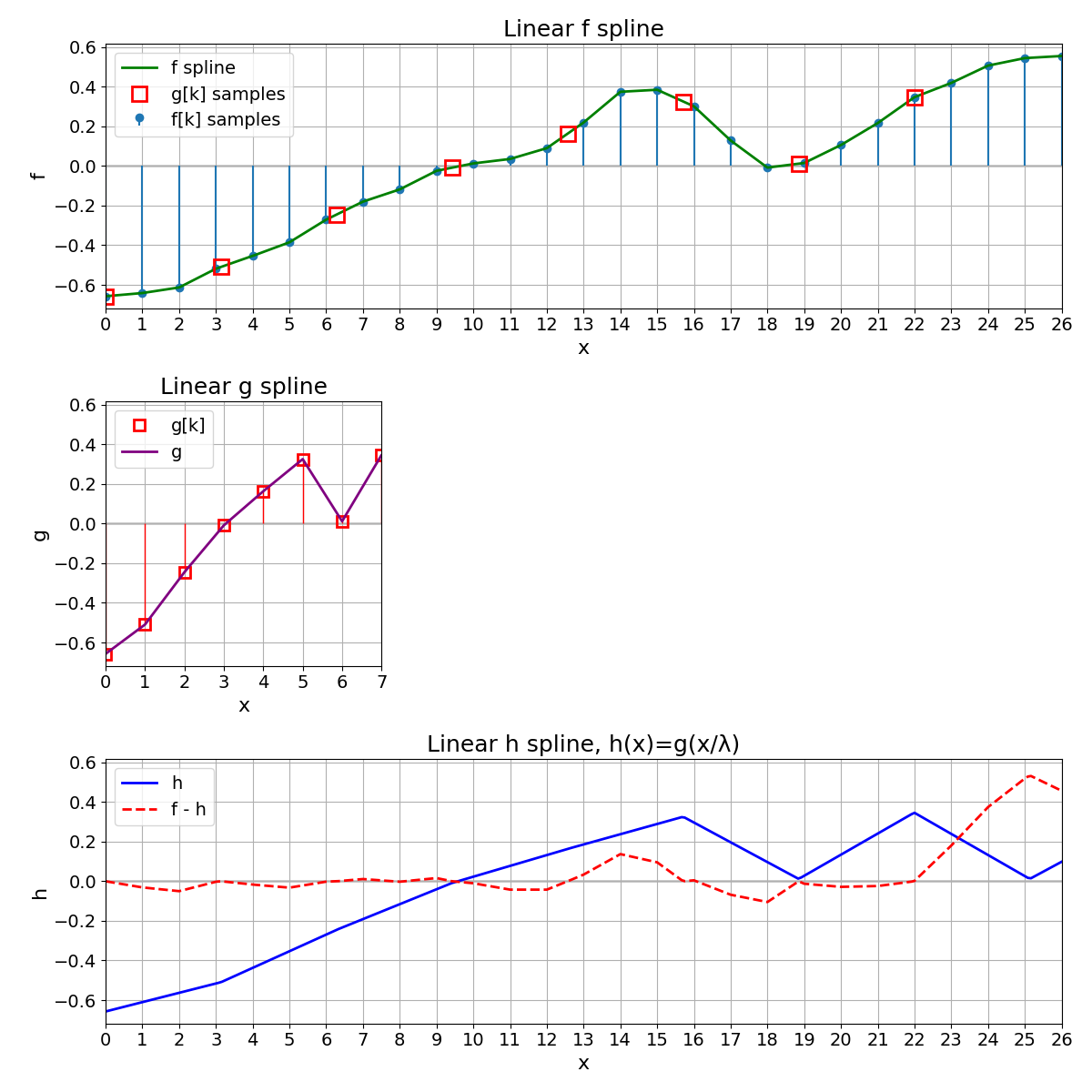
Variation with Linear Splines#
We repeat exactly everything with linear splines. As the MSE increases, we conclude that splines of degree 3 provide a better representation of the original signal than splines of degree 1.
base = "bspline1"
mode = "mirror"

# 1) Rebuild linear-spline version of f, then g
f_lin = TensorSpline(data=f_samples, coordinates=f_support, bases=base, modes=mode)
g_lin_samps = f_lin(coordinates=(f_resampled_coords,), grid=False)
g_lin = TensorSpline(data=g_lin_samps, coordinates=g_support, bases=base, modes=mode)

# 2) Evaluate them at the same plotting coordinates
f_lin_f = f_lin(coordinates=(f_coords,), grid=False)               # f_lin over domain 0..(K-1)
g_lin_g = g_lin(coordinates=(g_coords,), grid=False)               # g_lin over domain 0..(g_support_length-1)
h_lin_h = g_lin(coordinates=(f_coords / val_lambda,), grid=False)  # h_lin(x)=g_lin(x/λ) over 0..(K-1)

# 3) Create the 3×2 figure layout
fig3 = plt.figure(figsize=(12, 12))
gs3 = GridSpec(
    nrows=3,
    ncols=2,
    width_ratios=[g_support_length, f_support_length - g_support_length],
    height_ratios=[1, 1, 1]
)

# TOP ROW: entire row (two columns combined) for f
ax_top = fig3.add_subplot(gs3[0, :])
ax_top.set_title("Linear f spline")

# Plot f[k] as stems
ax_top.stem(f_support, f_samples, basefmt=" ", label="f[k] samples")

# Plot f spline
ax_top.plot(f_coords, f_lin_f, color="green", linewidth=2, label="f spline")

# Overplot discrete g[k] as unfilled red squares at x = k * val_lambda
x_g = np.arange(g_support_length) * val_lambda
ax_top.plot(
    x_g, g_lin_samps,
    "rs",              # red squares
    mfc='none',        # unfilled
    markersize=12,
    markeredgewidth=2,
    label="g[k] samples"
)

ax_top.axhline(0, color='black', linewidth=1, zorder=0)
ax_top.set_xlim(0, f_support_length - 1)
ax_top.set_xticks(np.arange(0, f_support_length, 1))
ax_top.set_xlabel("x")
ax_top.set_ylabel("f")
ax_top.grid(True)
ax_top.legend()

# MIDDLE ROW: left subplot shows g domain, right subplot is blank
ax_mid_left = fig3.add_subplot(gs3[1, 0])
ax_mid_right = fig3.add_subplot(gs3[1, 1])
ax_mid_right.axis("off")  # keep right side blank

ax_mid_left.set_title("Linear g spline")

# Discrete g[k] with stems
ax_mid_left.vlines(
    x=g_support,
    ymin=0,
    ymax=g_lin_samps,
    color='red',
    linewidth=1
)
ax_mid_left.plot(
    g_support,
    g_lin_samps,
    "rs", mfc='none', markersize=8, markeredgewidth=2,
    label="g[k]"
)
# g spline
ax_mid_left.plot(
    g_coords,
    g_lin_g,
    color="purple", linewidth=2,
    label="g"
)
ax_mid_left.axhline(0, color='black', linewidth=1, zorder=0)
ax_mid_left.set_xlim(0, g_support_length - 1)
ax_mid_left.set_xticks(np.arange(0, g_support_length, 1))
ax_mid_left.set_xlabel("x")
ax_mid_left.set_ylabel("g")
ax_mid_left.grid(True)
ax_mid_left.legend()
# Match y-range with top
ax_mid_left.set_ylim(ax_top.get_ylim())

# BOTTOM ROW: entire row for h
ax_bottom = fig3.add_subplot(gs3[2, :])
ax_bottom.set_title("Linear h spline, h(x)=g(x/λ)")

ax_bottom.plot(f_coords, h_lin_h, color="blue", linewidth=2, label="h")

# Evaluate f_lin at the same coords, then difference
f_lin_for_diff = f_lin(coordinates=(f_coords,), grid=False)
diff_lin = f_lin_for_diff - h_lin_h

# Plot difference in red, dashed
ax_bottom.plot(f_coords, diff_lin, color="red", linestyle="--", linewidth=2, label="f - h")

ax_bottom.axhline(0, color='black', linewidth=1, zorder=0)
ax_bottom.set_xlim(0, f_support_length - 1)
ax_bottom.set_xticks(np.arange(0, f_support_length, 1))
ax_bottom.set_xlabel("x")
ax_bottom.set_ylabel("h")
ax_bottom.grid(True)
ax_bottom.legend()
ax_bottom.set_ylim(ax_top.get_ylim())

fig3.tight_layout()
plt.show()

# 4) Recompute MSE with linear splines using midpoint rule
N = 1000
padding_fraction = 0.2 # We avoid artifacts near the edges by excluding part of the domain from each side
a = (f_support_length - 1) * padding_fraction
b = (f_support_length - 1) * (1 - padding_fraction)
dx = (b - a) / N

# mid_x are the midpoints of each subinterval
mid_x = np.linspace(a + dx/2, b - dx/2, N)

# Evaluate f_lin and h_lin at midpoints
f_lin_mid = f_lin(coordinates=(mid_x,), grid=False)
h_lin_mid = g_lin(coordinates=(mid_x / val_lambda,), grid=False)

# Midpoint Riemann sum for ∫(f_lin - h_lin)²
squared_diff_lin = (f_lin_mid - h_lin_mid) ** 2
integral_value_lin = np.sum(squared_diff_lin) * dx

# Divide by (b - a) to get MSE
mse_lin_midpoint = integral_value_lin / (b - a)
print(f"MSE with linear splines = {mse_lin_midpoint:.6e}")
MSE with linear splines = 2.604823e-03
Total running time of the script: (0 minutes 1.358 seconds)