Adaptive Regression Splines Module#

This example shows how to fit a piecewise-linear, knot-sparse model to 1-D data using the adaptive regression splines module.

What we do#

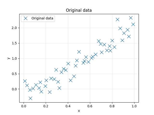
Visualize the raw data ((x,y)).
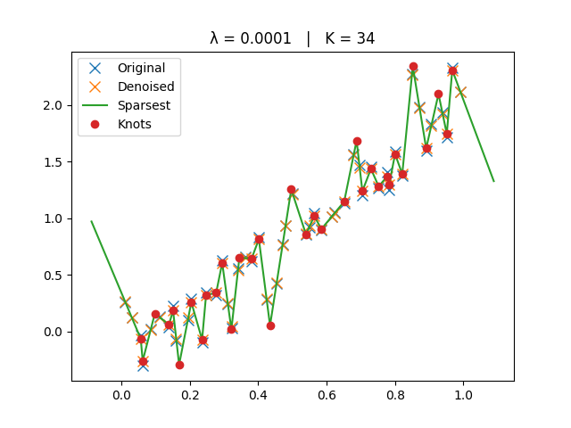
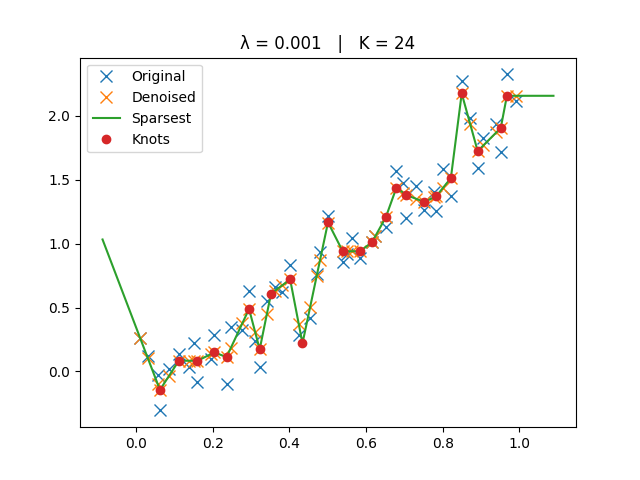
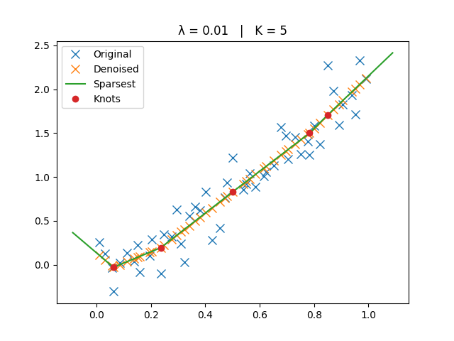
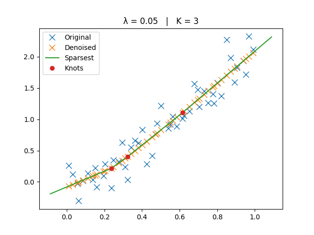
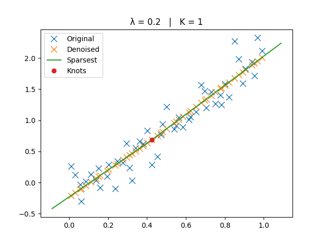
Denoise the samples by solving a TV-regularized least-squares problem on the second derivative:

\[\min_f \sum_i (f(x_i) - y_i)^2 \;+\; \lambda\,\|\mathrm{D}^2 f\|_{\mathcal{M}}.\]

This promotes piecewise-linear solutions with few breakpoints (knots).
From the denoised samples, extract the sparsest linear spline (fewest knots) with sparsest_interpolant(), and evaluate it with linear_spline().
Sweep λ over several values to illustrate the fidelity-sparsity trade-off. Each plot title reports the number of knots \(K\).

Notes#

Smaller \(\lambda\) → closer to interpolation (more knots).
Larger \(\lambda\) → smoother trend (fewer knots, eventually a line).
The helper cell below runs the full pipeline for any given \(\lambda\).

Imports#

import numpy as np
from matplotlib import pyplot as plt

from splineops.adaptive_regression_splines.denoising import denoise_y
from splineops.adaptive_regression_splines.sparsification import sparsest_interpolant, linear_spline

Data Preparation#

Create a dataset as (x,y) coordinates.

# Directly embedded data
data = np.array([
    [0.0107766212868331, 0.260227935166001],
    [0.0310564395737153, 0.124128829346261],
    [0.0568406178471921, -0.0319625924377939],
    [0.0624834663023982, -0.305487158118621],
    [0.0855836735802228, 0.0198584921896104],
    [0.111715185429166, 0.132374842819488],
    [0.139391914966393, 0.0346881909310438],
    [0.151220604385114, 0.225044726396834],
    [0.160372945787459, -0.0839333693634482],
    [0.196012653453612, 0.100524891786437],
    [0.20465948547682, 0.286553206119747],
    [0.236142103912376, -0.0969023194982265],
    [0.247757212881283, 0.344416030734225],
    [0.277270837091189, 0.322338105021903],
    [0.294942432854744, 0.628493233708394],
    [0.311124804679808, 0.238685146788896],
    [0.322729104513214, 0.0314182350548619],
    [0.341198353790244, 0.554001442697049],
    [0.362426869114815, 0.658491185386012],
    [0.380891037570895, 0.622866466731061],
    [0.402149882582122, 0.832680133314763],
    [0.424514186772157, 0.282871329344068],
    [0.454259779607654, 0.418961645149398],
    [0.471194339641083, 0.765569673816136],
    [0.480251119603182, 0.936269519087734],
    [0.50143948559379, 1.21690697362292],
    [0.539345526600005, 0.856785149480669],
    [0.551362009238399, 0.918563536364133],
    [0.56406586469322, 1.04369945227154],
    [0.585046514891406, 0.891659244596406],
    [0.614876517081502, 1.01020862285029],
    [0.623908589622186, 1.05646068606692],
    [0.651627178545465, 1.13455056187785],
    [0.679400399781766, 1.56682321923577],
    [0.696936576029801, 1.47238622944877],
    [0.704796955182952, 1.20492985044235],
    [0.729875394285375, 1.45329058102288],
    [0.752399114367628, 1.26394538858847],
    [0.776579617991004, 1.4052754431186],
    [0.783135827892922, 1.2534612824523],
    [0.800371524043548, 1.58782975330571],
    [0.821400442874384, 1.3740621261335],
    [0.849726902218741, 2.27247168443063],
    [0.872126589233067, 1.98304748773148],
    [0.89137702874173, 1.59274379691406],
    [0.906347248186443, 1.82991582958117],
    [0.939772323088249, 1.9344157693364],
    [0.951594904384916, 1.71570985938051],
    [0.967602823452471, 2.32573940626424],
    [0.991018964382358, 2.11540602201059]
])

x, y = data[:, 0], data[:, 1]

fig, ax = plt.subplots()
ax.plot(x, y, 'x', label='Original data', markersize=10)
ax.set_title("Original data")
ax.set_xlabel("x")
ax.set_ylabel("y")
ax.grid(True, alpha=0.3)
ax.legend()
plt.show()

Helpers#

The original, denoised, and sparsest spline solutions are plotted for comparison.

# Helper for lambda sweeps (one-time cell)
def _run_lambda(lamb: float):
    y_d = denoise_y(x, y, lamb, rho=lamb)
    knots, amplitudes, polynomial = sparsest_interpolant(x, y_d)

    margin = (x[-1] - x[0]) / 10
    t_grid = np.concatenate(([x[0] - margin], knots, [x[-1] + margin]))

    fig, ax = plt.subplots()
    ax.plot(x, y, 'x', label='Original', markersize=8)
    ax.plot(x, y_d, 'x', label='Denoised', markersize=8)
    ax.plot(t_grid, linear_spline(t_grid, knots, amplitudes, polynomial), label='Sparsest')
    if len(knots) > 0:
        ax.plot(knots, linear_spline(knots, knots, amplitudes, polynomial), 'o', color="C3", label='Knots')
    ax.set_title(f"λ = {lamb:g}   |   K = {len(knots)}")
    ax.legend()
    plt.show()