Spline Bases

Plotting the spline bases of the library and several transformations and operations.

Imports and Utilities

Define helper functions to visualize the spline bases and derived splines.

import numpy as np
import matplotlib.pyplot as plt
from splineops.spline_interpolation.bases.utils import create_basis

# Common x-grid for basis functions
x_values = np.linspace(-3, 3, 1000)


def plot_lines_1d(
    x,
    ys,
    title,
    labels=None,
    xlabel="x",
    ylabel="y",
    figsize=(8, 4),
    xlim=None,
    ylim=None,
    show_legend=False,
    tight_layout=False,
):
    """Generic helper to plot one or several 1D curves."""
    plt.figure(figsize=figsize)

    # Accept a single array or a list/tuple
    if not isinstance(ys, (list, tuple)):
        ys = [ys]

    for i, y in enumerate(ys):
        kwargs = {}
        if labels is not None and i < len(labels):
            kwargs["label"] = labels[i]
        plt.plot(x, y, **kwargs)

    if xlim is not None:
        plt.xlim(*xlim)
    if ylim is not None:
        plt.ylim(*ylim)

    plt.grid(True)
    plt.xlabel(xlabel)
    plt.ylabel(ylabel)
    plt.title(title)

    if show_legend and labels is not None:
        plt.legend()

    if tight_layout:
        plt.tight_layout()

    plt.show()


def plot_bases(names, x_values, title, show_legend=True):
    """Plot several spline bases using the generic 1D plotting helper."""
    ys = []
    labels = []

    for name in names:
        if name == "keys":
            readable_name = "Keys Spline"
        else:
            name_parts = name.split("-")
            readable_name = f"{name_parts[0][:-1]} degree {name_parts[0][-1]}"
        ys.append(create_basis(name).eval(x_values))
        labels.append(readable_name)

    plot_lines_1d(
        x=x_values,
        ys=ys,
        labels=labels,
        title=title,
        figsize=(12, 6),
        show_legend=show_legend,
    )

Bases

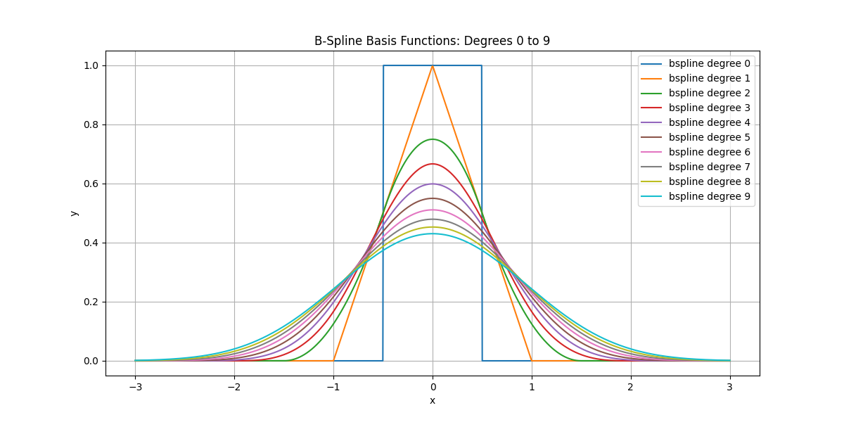
B-Spline Bases

Plot B-spline basis functions for degree 0 to 9.

plot_bases(
    names=[f"bspline{i}" for i in range(10)],
    x_values=x_values,
    title="B-Spline Basis Functions: Degrees 0 to 9",
)

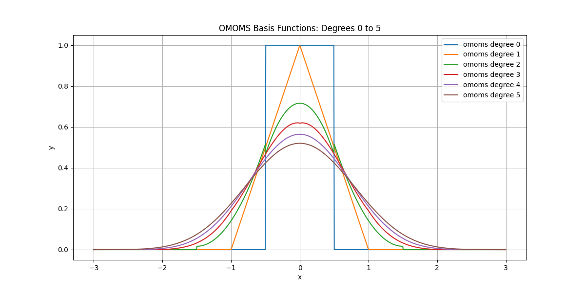
OMOMS Bases

Plot OMOMS basis functions for degree 0 to 5.

plot_bases(
    names=[f"omoms{i}" for i in range(6)],
    x_values=x_values,
    title="OMOMS Basis Functions: Degrees 0 to 5",
)

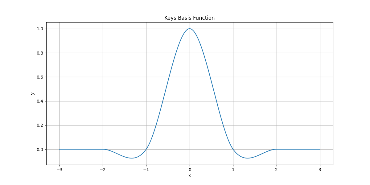
Keys Basis

Plot the Keys basis function (legend omitted, title is enough).

plot_bases(
    names=["keys"],
    x_values=x_values,
    title="Keys Basis Function",
    show_legend=False,
)

Transforming Cubic B-Splines

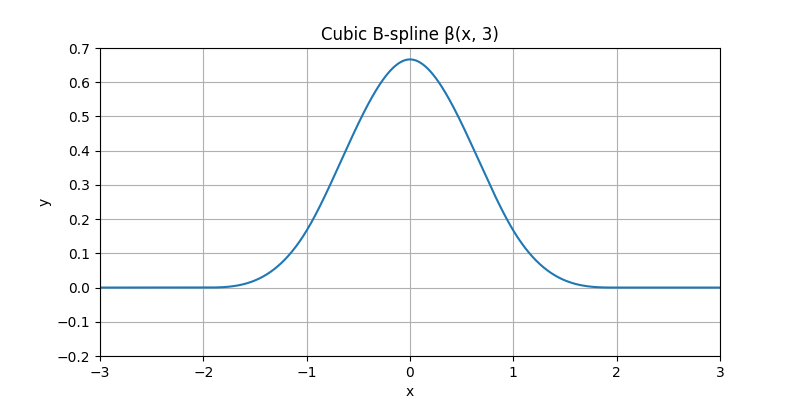
Helper for Cubic B-Spline

beta3_basis = create_basis("bspline3")


def beta3(x):
    """Centered cubic B-spline β(x, 3)."""
    return beta3_basis.eval(x)

Single Cubic B-Spline

Start from the centered cubic B-spline β(x, 3), which is the basic building block for the following plots.

plot_lines_1d(
    x=x_values,
    ys=beta3(x_values),
    title="Cubic B-spline β(x, 3)",
    xlim=(-3, 3),
    ylim=(-0.2, 0.7),
)

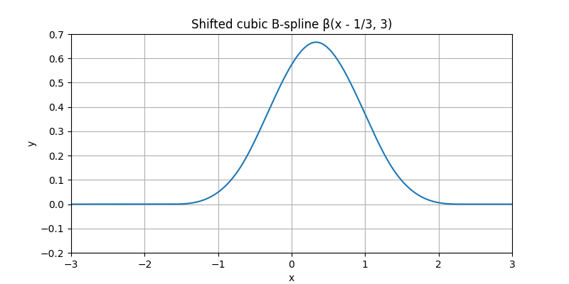
Shifted Cubic B-Spline

Shift the cubic B-spline horizontally by one third. This only affects the argument of β, not its shape.

shift = 1.0 / 3.0

plot_lines_1d(
    x=x_values,
    ys=beta3(x_values - shift),
    title="Shifted cubic B-spline β(x - 1/3, 3)",
    xlim=(-3, 3),
    ylim=(-0.2, 0.7),
)

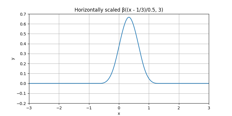
Shrunk Cubic B-Spline

Shrink the spline horizontally by 60%. This is done by scaling the argument of β, which changes the effective width of its support.

shift = 1.0 / 3.0
scale = 0.5   # same as "/ 0.5" in the text

plot_lines_1d(
    x=x_values,
    ys=beta3((x_values - shift) / scale),
    title="Horizontally scaled β((x - 1/3)/0.5, 3)",
    xlim=(-3, 3),
    ylim=(-0.2, 0.7),
)

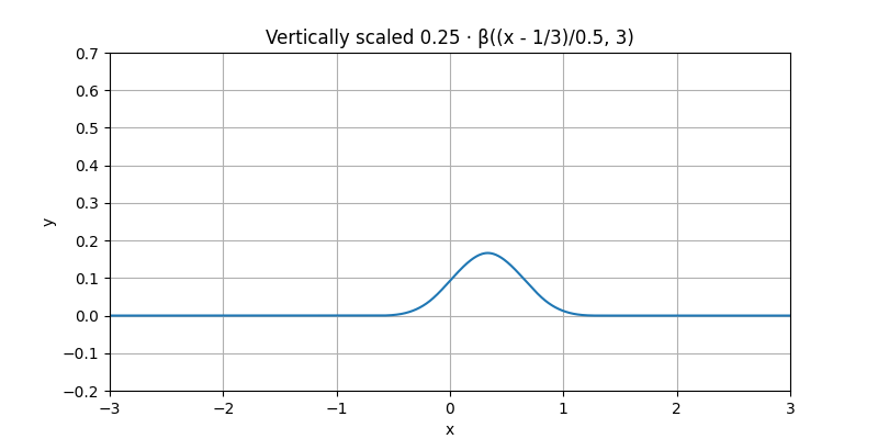
Weighted Cubic B-Spline

Multiply the shrunk and shifted spline by a constant factor. This operation is called weighting.

shift = 1.0 / 3.0
scale = 0.5
amp = 0.25

plot_lines_1d(
    x=x_values,
    ys=amp * beta3((x_values - shift) / scale),
    title="Vertically scaled 0.25 · β((x - 1/3)/0.5, 3)",
    xlim=(-3, 3),
    ylim=(-0.2, 0.7),
)

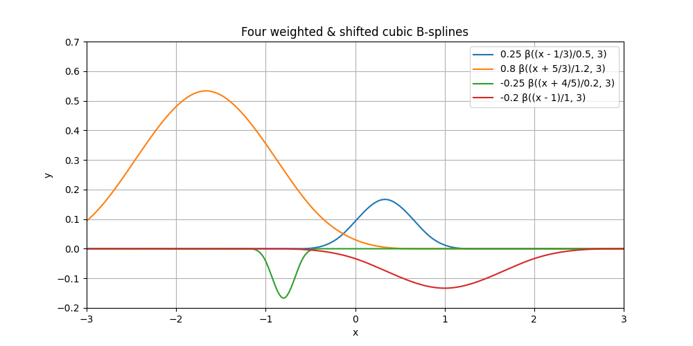
Several Transformed B-Splines

Use several combinations of (shift, shrink, weight) to obtain different functions, all of which are still cubic B-splines up to their parameters.

def beta3_shift_scale(x, shift, scale, amp=1.0):
    """Shift, scale, and weight the cubic B-spline."""
    return amp * beta3((x + shift) / scale)


curves = [
    ("0.25 β((x - 1/3)/0.5, 3)",
     lambda x: beta3_shift_scale(x, shift=-1.0/3.0, scale=0.5, amp=0.25)),
    ("0.8 β((x + 5/3)/1.2, 3)",
     lambda x: beta3_shift_scale(x, shift=+5.0/3.0, scale=1.2, amp=0.8)),
    ("-0.25 β((x + 4/5)/0.2, 3)",
     lambda x: beta3_shift_scale(x, shift=+4.0/5.0, scale=0.2, amp=-0.25)),
    ("-0.2 β((x - 1)/1, 3)",
     lambda x: beta3_shift_scale(x, shift=-1.0, scale=1.0, amp=-0.2)),
]

plot_lines_1d(
    x=x_values,
    ys=[f(x_values) for _, f in curves],
    labels=[label for label, _ in curves],
    title="Four weighted & shifted cubic B-splines",
    figsize=(10, 5),
    xlim=(-3, 3),
    ylim=(-0.2, 0.7),
    show_legend=True,
)

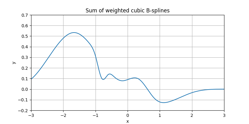
Sum of B-Splines

Sum these functions together to obtain a new combined function. It is built from cubic B-splines but is itself no longer a basis function.

def combined_spline(x):
    return sum(f(x) for _, f in curves)

plot_lines_1d(
    x=x_values,
    ys=combined_spline(x_values),
    title="Sum of weighted cubic B-splines",
    xlim=(-3, 3),
    ylim=(-0.2, 0.7),
)

Building Splines

Helpers for Spline Decomposition

These helpers are used for the uniform spline, its samples, and their decomposition into shifted and weighted cubic B-splines.

# Integer shifts k = -4, ..., 4
k_vals = np.arange(-4, 5)

# Same coefficients as in the original notebook:
coeffs = np.array([-2, -3, 4, 1, -5, -1, 2, 6, -4], dtype=float)

def spline_from_coeffs(x):
    """Uniform spline f(x) = Σ_k c[k] β³(x - k)."""
    x = np.asarray(x)
    y = np.zeros_like(x, dtype=float)
    for k, ck in zip(k_vals, coeffs):
        y += ck * beta3(x - k)
    return y

def spline_term(k, x):
    """Single term c[k] β³(x - k) for integer k in [-4, 4]."""
    return coeffs[k + 4] * beta3(x - k)

# Common grids for these examples
x_plot = np.linspace(-3.1, 3.1, 2000)
x_samples = np.arange(-3, 4)  # integer sample positions

def spline_samples():
    """Return integer sample positions and corresponding spline values."""
    return x_samples, spline_from_coeffs(x_samples)

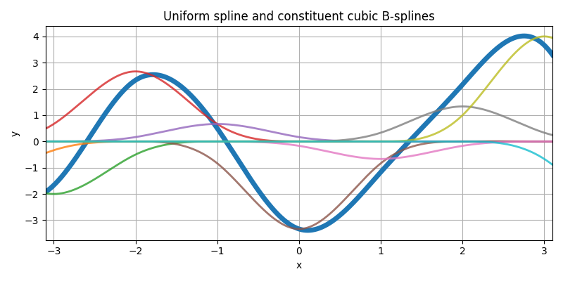
Sum of Shifted Cubic B-Splines

Build a regular (uniform) spline as

f(x) = Σ_k c[k] β³(x - k),

using integer shifts and fixed coefficients c[k]. The thick curve is the full spline; the thin curves are the individual terms c[k] β³(x - k).

plt.figure(figsize=(8, 4))

# Thick combined spline
plt.plot(
    x_plot,
    spline_from_coeffs(x_plot),
    linewidth=5,
)

# Thin constituent terms c[k] β³(x - k)
for k in k_vals:
    plt.plot(
        x_plot,
        spline_term(k, x_plot),
        linewidth=2,
        alpha=0.8,
    )

plt.xlim(-3.1, 3.1)
plt.grid(True)
plt.xlabel("x")
plt.ylabel("y")
plt.title("Uniform spline and constituent cubic B-splines")
plt.tight_layout()
plt.show()

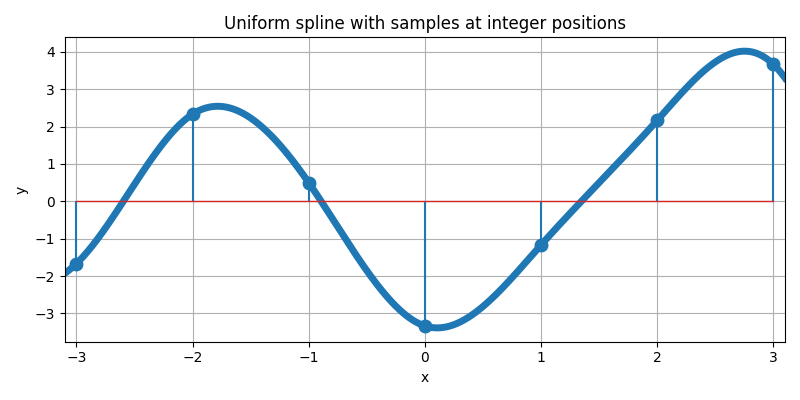
Sampling a Spline

Sample the spline at integer locations x = k. These samples define a discrete sequence f[k] that we may want to reconstruct from a spline interpolant.

x_samp, y_samp = spline_samples()

plt.figure(figsize=(8, 4))

# Thick spline
plt.plot(
    x_plot,
    spline_from_coeffs(x_plot),
    linewidth=5,
)

# Stems + markers for samples
markerline, stemlines, baseline = plt.stem(x_samp, y_samp)
plt.setp(markerline, markersize=9)
plt.setp(stemlines, linewidth=1.5)
plt.setp(baseline, linewidth=1.0)

plt.xlim(-3.1, 3.1)
plt.grid(True)
plt.xlabel("x")
plt.ylabel("y")
plt.title("Uniform spline with samples at integer positions")
plt.tight_layout()
plt.show()

From Samples to Splines

Illustrate the relationship between:

• the discrete samples f[k] (left),

• the shifted and weighted basis functions c[k] β³(x - k) (middle),

• and the resulting spline f(x) that interpolates the samples (right).

x_samp, y_samp = spline_samples()

fig, axes = plt.subplots(1, 3, figsize=(12, 4), sharey=True)

# Left panel: samples only
ax = axes[0]
markerline, stemlines, baseline = ax.stem(x_samp, y_samp)
plt.setp(markerline, markersize=9)
plt.setp(stemlines, linewidth=1.5)
plt.setp(baseline, linewidth=1.0)

ax.set_xlim(-3.1, 3.1)
ax.grid(True)
ax.set_xlabel("x")
ax.set_ylabel("y")
ax.set_title("Samples f[k]")

# Middle panel: basis terms + samples
ax = axes[1]

for k in k_vals:
    ax.plot(
        x_plot,
        spline_term(k, x_plot),
        linewidth=2,
        alpha=0.8,
    )

markerline, stemlines, baseline = ax.stem(x_samp, y_samp)
plt.setp(markerline, markersize=9)
plt.setp(stemlines, linewidth=1.5)
plt.setp(baseline, linewidth=1.0)

ax.set_xlim(-3.1, 3.1)
ax.grid(True)
ax.set_xlabel("x")
ax.set_title(r"Weighted terms $c[k]\beta^3(x-k)$")

# Right panel: full spline + terms + samples
ax = axes[2]

ax.plot(
    x_plot,
    spline_from_coeffs(x_plot),
    linewidth=5,
)

for k in k_vals:
    ax.plot(
        x_plot,
        spline_term(k, x_plot),
        linewidth=2,
        alpha=0.8,
    )

markerline, stemlines, baseline = ax.stem(x_samp, y_samp)
plt.setp(markerline, markersize=9)
plt.setp(stemlines, linewidth=1.5)
plt.setp(baseline, linewidth=1.0)

ax.set_xlim(-3.1, 3.1)
ax.grid(True)
ax.set_xlabel("x")
ax.set_title("Resulting spline f(x)")

plt.tight_layout()
plt.show()