Resample a 1D Spline

Resample a 1D spline with different sampling rate.

1. Assume that a user-provided 1D list of samples \(f[k]\) has been obtained by sampling a spline on a unit grid.

2. From the samples, recover the continuously defined spline \(f(x)\).

3. Resample \(f(x)\) to get \(g[k] = f(Tk)\), with \(|T| > 1\).

4. Create a new spline \(g(x)\) from the samples \(g[k]\).

Imports

import numpy as np
import matplotlib.pyplot as plt
from matplotlib.gridspec import GridSpec
from splineops.spline_interpolation.tensor_spline import TensorSpline
from splineops.spline_interpolation.bases.utils import create_basis

plt.rcParams.update({
    "font.size": 14,     # Base font size
    "axes.titlesize": 18,  # Title font size
    "axes.labelsize": 16,  # Label font size
    "xtick.labelsize": 14,
    "ytick.labelsize": 14
})

Initial 1D Samples

Define a 1D discrete signal \(f[k]\) on a unit grid, which we will treat as samples of an underlying spline.

number_of_samples = 27

f_support = np.arange(number_of_samples, dtype=np.float64)
f_support_length = len(f_support)  # == number_of_samples

f_samples = np.array([
    -0.657391, -0.641319, -0.613081, -0.518523, -0.453829, -0.385138,
    -0.270688, -0.179849, -0.11805, -0.0243016, 0.0130667, 0.0355389,
    0.0901577, 0.219599, 0.374669, 0.384896, 0.301386, 0.128646,
    -0.00811776, 0.0153119, 0.106126, 0.21688, 0.347629, 0.419532,
    0.50695, 0.544767, 0.555373
], dtype=np.float64)

plot_points_per_unit = 12

# Interpolated signal
base = "bspline3"
mode = "mirror"

f = TensorSpline(data=f_samples, coordinates=f_support, bases=base, modes=mode)

f_coords = np.array([q / plot_points_per_unit
                     for q in range(plot_points_per_unit * f_support_length)])
f_data = f(coordinates=(f_coords,), grid=False)

Coarsening of f

Sample the fine spline \(f(x)\) on a coarser grid to obtain the new discrete sequence \(g[k] = f(Tk)\).

# Choose the number of coarse samples in the same way as the resize example
# (e.g., 8 for 27 // pi)
g_support_length = round(f_support_length // np.pi)

# Effective coarse spacing so that the first and last coarse nodes
# align with x = 0 and x = f_support_length - 1 (i.e., 0 and 26)
val_T = (f_support_length - 1) / (g_support_length - 1)

k = np.arange(g_support_length, dtype=np.float64)

# Physical positions where g is sampled from f: x = T * k
x_g = k * val_T
g_samples = f(coordinates=(x_g,), grid=False)

# Build g as a spline over PHYSICAL x (so markers align across plots)
g = TensorSpline(data=g_samples, coordinates=x_g, bases=base, modes=mode)

# Evaluate g across the full width of f (mirror padding extends toward the right)
g_coords_full = f_coords
g_data_full = g(coordinates=(g_coords_full,), grid=False)

# Preview: same content as the top row of the final 2-row plot
plt.figure(figsize=(12, 4))
ax = plt.gca()
ax.set_title("Interpolated f spline with coarse samples g[k]")
ax.stem(f_support, f_samples, basefmt=" ", label="f[k] samples")
ax.plot(f_coords, f_data, color="green", linewidth=2, label="f spline")

# Vertical red lines from 0 to g[k] at x = T*k (now thick)
ax.vlines(x=x_g, ymin=0, ymax=g_samples, color="red", linewidth=2.0)

# g[k] markers at x = T*k
ax.plot(
    x_g, g_samples, "rs",
    mfc="none", markersize=12, markeredgewidth=2, label="g[k] samples"
)

ax.axhline(0, color="black", linewidth=1, zorder=0)
ax.set_xlim(0, f_support_length - 1)
ax.set_xticks(np.arange(0, f_support_length, 1))  # show 0..26 on the axis
ax.set_xlabel("x")
ax.set_ylabel("f")
ax.grid(True)
ax.legend()

# --- Annotate one interval of length T between two g[k] samples ---
if g_support_length >= 2:
    # Prefer a later interval if possible:
    #  - third interval: between g[2] and g[3] if g_support_length >= 4
    #  - else second: between g[1] and g[2] if g_support_length >= 3
    #  - else first: between g[0] and g[1]
    if g_support_length >= 4:
        start_idx = 2  # interval between k=2 and k=3
    elif g_support_length >= 3:
        start_idx = 1  # interval between k=1 and k=2
    else:
        start_idx = 0  # only one interval available

    x_T_start = x_g[start_idx]
    x_T_end = x_g[start_idx + 1]

    # Place the annotation slightly above the x-axis
    ymin, ymax = ax.get_ylim()
    y_T = ymin + 0.1 * (ymax - ymin)

    # Red double arrow between the chosen g[k] samples
    ax.annotate(
        "",
        xy=(x_T_start, y_T),
        xytext=(x_T_end, y_T),
        arrowprops=dict(arrowstyle="<->", color="red", linewidth=1.5),
    )

    # Label "T" at the midpoint of the interval, also in red
    ax.text(
        0.5 * (x_T_start + x_T_end),
        y_T,
        "T",
        ha="center",
        va="bottom",
        fontsize=14,
        color="red",
    )

    # Emphasize that these two vertical lines are the boundaries of the T interval
    # by extending them across the full vertical range.
    ax.vlines(
        [x_T_start, x_T_end],
        ymin,
        ymax,
        color="red",
        linewidth=2.0,
        zorder=2,
    )

plt.tight_layout()
plt.show()

Coarse-Grid Basis Functions

Compare the shifted basis functions on the fine grid \(V_1\) and on the coarse grid \(V_T\). On the fine grid, the coefficients \(c[k]\) weight \(\varphi(x - k)\). On the coarse grid, the coefficients \(c_T[k]\) weight \(\varphi(x/T - k)\). In this example, \(\varphi = \beta^{3}\) is the cubic B-spline.

# Retrieve the true spline coefficients for f (fine grid) and g (coarse grid)
f_coeffs = f.coefficients
g_coeffs = g.coefficients

# Basis function corresponding to `base` (e.g. "bspline3")
basis = create_basis(base)

# Dense x-grids: fine grid for f, coarse-domain grid for g
x_dense_fine = f_coords        # dense sampling of f(x) on [0, K-1]
x_dense_coarse = g_coords_full  # same physical domain, used for g(x)

fig = plt.figure(figsize=(12, 8))
gs = GridSpec(nrows=2, ncols=1, height_ratios=[1, 1])

# --- TOP: fine-grid basis functions (V1) ---
ax_top = fig.add_subplot(gs[0, 0])
ax_top.set_title("f[k] samples with shifted basis functions")

# Plot f[k] samples as stems on the integer grid
ax_top.stem(f_support, f_samples, basefmt=" ", label="f[k] samples")

# Overlay fine-grid basis functions: c[k] · ϕ(x − k)
for k_idx, c_k in enumerate(f_coeffs):
    y_basis = c_k * basis.eval(x_dense_fine - k_idx)
    ax_top.plot(x_dense_fine, y_basis, linewidth=2, alpha=0.7)

ax_top.axhline(0, color="black", linewidth=1, zorder=0)
ax_top.set_xlim(0, f_support_length - 1)
ax_top.set_xticks(np.arange(0, f_support_length, 1))
ax_top.set_ylabel("Amplitude")
ax_top.grid(True)
ax_top.legend()

# --- BOTTOM: coarse-grid basis functions (V_T) ---
ax_bottom = fig.add_subplot(gs[1, 0])
ax_bottom.set_title("g[k] samples with resized shifted basis functions")

# Coarse samples g[k] at x = T*k
ax_bottom.vlines(x=x_g, ymin=0, ymax=g_samples, color="red", linewidth=2.0)
ax_bottom.plot(
    x_g, g_samples, "rs",
    mfc="none", markersize=12, markeredgewidth=2, label="g[k] samples"
)

# Overlay coarse-grid basis functions: c_T[k] · ϕ(x/T − k)
for k_idx, c_k in enumerate(g_coeffs):
    y_basis = c_k * basis.eval(x_dense_coarse / val_T - k_idx)
    ax_bottom.plot(x_dense_coarse, y_basis, linewidth=2, alpha=0.7)

ax_bottom.axhline(0, color="black", linewidth=1, zorder=0)
ax_bottom.set_xlim(0, f_support_length - 1)
ax_bottom.set_ylabel("Amplitude")
ax_bottom.grid(True)

# Use coarse-grid ticks (x = kT) with labels k on the bottom axis
max_k_tick = int(np.floor((f_support_length - 1) / val_T))
tick_ks = np.arange(max_k_tick + 1)          # coarse indices k = 0,1,...
tick_positions = tick_ks * val_T            # physical positions x = kT
ax_bottom.set_xticks(tick_positions)
ax_bottom.set_xticklabels([str(k) for k in tick_ks])
ax_bottom.set_xlabel("x")

ax_bottom.legend()
plt.tight_layout()
plt.show()

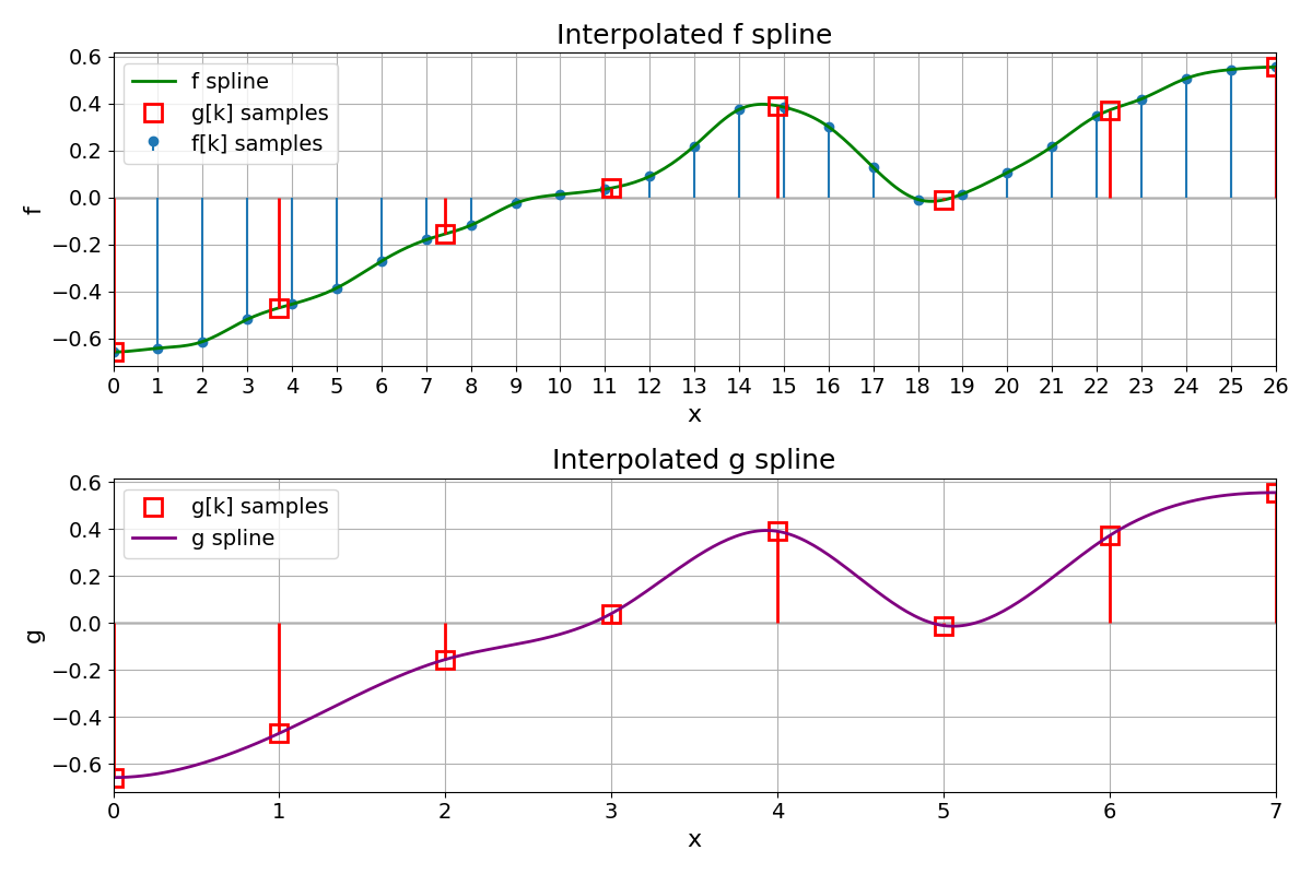
Spline g

Compare the original spline \(f\) and the coarse spline g on the same physical domain, using the coarse grid on the x-axis.

fig = plt.figure(figsize=(12, 8))
gs = GridSpec(nrows=2, ncols=1, height_ratios=[1, 1])

# Top: full width with x in 0..26
ax_top = fig.add_subplot(gs[0, 0])

# Bottom: full width with x in 0..26 (own ticks so we can label at multiples of T)
ax_bottom = fig.add_subplot(gs[1, 0])

# --- TOP: f[k] + f(x) + g[k] markers at x = T*k ---
ax_top.set_title("Interpolated f spline")
ax_top.stem(f_support, f_samples, basefmt=" ", label="f[k] samples")
ax_top.plot(f_coords, f_data, color="green", linewidth=2, label="f spline")

# Red lines from 0 to g[k] at x = T*k (match thickness used above)
ax_top.vlines(x=x_g, ymin=0, ymax=g_samples, color="red", linewidth=2.0)

# g[k] markers at x = T*k
ax_top.plot(
    x_g, g_samples, "rs",
    mfc="none", markersize=12, markeredgewidth=2, label="g[k] samples"
)

ax_top.axhline(0, color="black", linewidth=1, zorder=0)
ax_top.set_xlim(0, f_support_length - 1)
ax_top.set_xticks(np.arange(0, f_support_length, 1))  # show 0..26 on the top axis
ax_top.set_xlabel("x")
ax_top.set_ylabel("f")
ax_top.grid(True)
ax_top.legend()

# --- BOTTOM: g[k] + g(x) across full width; x-axis is uniform in k at multiples of T ---
ax_bottom.set_title("Interpolated g spline")
ax_bottom.vlines(x=x_g, ymin=0, ymax=g_samples, color="red", linewidth=2.0)
ax_bottom.plot(
    x_g, g_samples, "rs",
    mfc="none", markersize=12, markeredgewidth=2, label="g[k] samples"
)
ax_bottom.plot(g_coords_full, g_data_full, color="purple", linewidth=2, label="g spline")

ax_bottom.axhline(0, color="black", linewidth=1, zorder=0)
ax_bottom.set_xlim(0, f_support_length - 1)
ax_bottom.set_ylabel("g")
ax_bottom.grid(True)
ax_bottom.legend()
ax_bottom.set_ylim(ax_top.get_ylim())  # optional: match vertical scale

# Bottom ticks at every multiple of T that fits (e.g., k = 0..8 for length 27)
max_k_tick = int(np.floor((f_support_length - 1) / val_T))
tick_ks = np.arange(max_k_tick + 1)  # e.g., 0..8
tick_positions = tick_ks * val_T
ax_bottom.set_xticks(tick_positions)
ax_bottom.set_xticklabels([str(k) for k in tick_ks])
ax_bottom.set_xlabel("x")

fig.tight_layout()
plt.show()