Resample a 1D spline

Resample a 1D spline with different sampling rate.

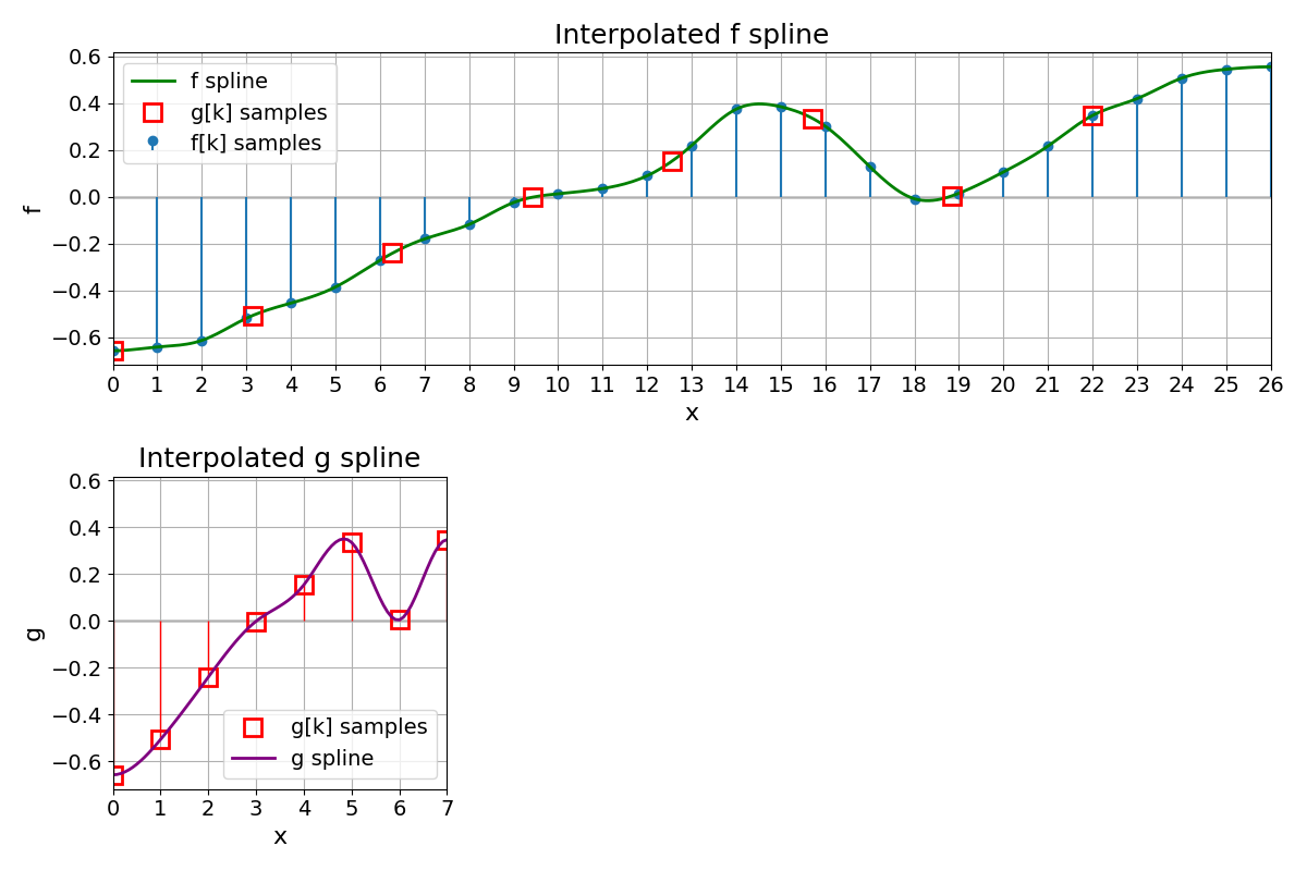
1. Assume that a user-provided 1D list of samples \(f[k]\) has been obtained by sampling a spline on a unit grid.

2. From the samples, recover the continuously defined spline \(f(x)\).

3. Resample \(f(x)\) to get \(g[k] = f(Tk)\), with \(|T| > 1\).

4. Create a new spline \(g(x)\) from the samples \(g[k]\).

Imports

import numpy as np
import matplotlib.pyplot as plt
from matplotlib.gridspec import GridSpec
from splineops.interpolate.tensorspline import TensorSpline

plt.rcParams.update({
    "font.size": 14,     # Base font size
    "axes.titlesize": 18,  # Title font size
    "axes.labelsize": 16,  # Label font size
    "xtick.labelsize": 14,
    "ytick.labelsize": 14
})

Initial 1D Samples

We generate 1D samples and treat them as discrete signal points.

Let \(\mathbf{f} = (f[0], f[1], f[2], \dots, f[K-1])\) be a 1D array of data.

These are the input samples that we are going to interpolate.

number_of_samples = 27

f_support = np.arange(number_of_samples)
f_support_length = len(f_support) # It's equal to number_of_samples

f_samples = np.array([
    -0.657391, -0.641319, -0.613081, -0.518523, -0.453829, -0.385138,
    -0.270688, -0.179849, -0.11805, -0.0243016, 0.0130667, 0.0355389,
    0.0901577, 0.219599, 0.374669, 0.384896, 0.301386, 0.128646,
    -0.00811776, 0.0153119, 0.106126, 0.21688, 0.347629, 0.419532,
    0.50695, 0.544767, 0.555373
])

plot_points_per_unit = 12

# Interpolated signal
base = "bspline3"
mode = "mirror"

f = TensorSpline(data=f_samples, coordinates=f_support, bases=base, modes=mode)

f_coords = np.array([q / plot_points_per_unit
                        for q in range(plot_points_per_unit * f_support_length)])

# Syntax hint: pass (plot_coords,) not plot_coords
f_data = f(coordinates=(f_coords,), grid=False)

Coarsening of f

We define \(T\) with \(|T| > 1\) and sample \(f(x)\) at \(x = T k\) as

\[g[k] = f(T k).\]

These points \(g[k]\) form a new discrete set, which we then treat as a separate signal to build another spline \(g\).

val_T = np.pi

g_support_length = round(f_support_length // val_T)
g_support = np.arange(g_support_length)
f_resampled_coords = np.array([q * val_T for q in range(g_support_length)])
g_samples = f(coordinates=(f_resampled_coords,), grid=False)
g = TensorSpline(data=g_samples, coordinates=g_support, bases=base, modes=mode)

g_coords = np.array([q/plot_points_per_unit
                     for q in range(plot_points_per_unit * len(g_support))])
g_data = g(coordinates=(g_coords,), grid=False)

fig = plt.figure(figsize=(12, 8))

gs = GridSpec(
    nrows=2,
    ncols=2,
    # Match widths: first column = g_support_length, second column = leftover
    width_ratios=[g_support_length, f_support_length - g_support_length],
    height_ratios=[1, 1]
)

# Top row: entire row (two columns combined)
ax_top = fig.add_subplot(gs[0, :])

# Bottom row: left side for g, right side blank
ax_bottom_left = fig.add_subplot(gs[1, 0])
ax_bottom_right = fig.add_subplot(gs[1, 1])
ax_bottom_right.axis("off")  # leave right side blank

# 1) TOP ROW: f[k] + f spline + discrete g[k]
ax_top.set_title("Interpolated f spline")

# Plot discrete f[k] as stems
ax_top.stem(f_support, f_samples, basefmt=" ", label="f[k] samples")

# Plot spline f(x)
ax_top.plot(f_coords, f_data, color="green", linewidth=2, label="f spline")

# Overplot discrete g[k] as unfilled red squares at x = k * val_T
x_g = np.arange(g_support_length) * val_T
ax_top.plot(
    x_g,
    g_samples,
    "rs",              # red squares
    mfc='none',        # unfilled
    markersize=12,
    markeredgewidth=2,
    label="g[k] samples"
)

# Horizontal line at 0 for reference
ax_top.axhline(0, color='black', linewidth=1, zorder=0)

# Make sure the top axis goes from 0..(f_support_length-1)
ax_top.set_xlim(0, f_support_length - 1)
ax_top.set_xticks(np.arange(0, f_support_length, 1))
ax_top.set_xlabel("x")
ax_top.set_ylabel("f")
ax_top.grid(True)
ax_top.legend()

# 2) BOTTOM LEFT: discrete g[k] + g spline
ax_bottom_left.set_title("Interpolated g spline")

# Plot discrete g[k] with red vertical lines and unfilled red squares
ax_bottom_left.vlines(
    x=g_support,
    ymin=0,
    ymax=g_samples,
    color='red',
    linestyle='-',
    linewidth=1
)
ax_bottom_left.plot(
    g_support,
    g_samples,
    "rs",              # red squares
    mfc='none',        # unfilled
    markersize=12,
    markeredgewidth=2,
    label="g[k] samples"
)

# Plot g spline in purple over the same domain
ax_bottom_left.plot(
    g_coords,
    g_data,
    color="purple",
    linewidth=2,
    label="g spline"
)

# Horizontal line at 0
ax_bottom_left.axhline(0, color='black', linewidth=1, zorder=0)

ax_bottom_left.set_xlim(0, g_support_length - 1)
ax_bottom_left.set_xticks(np.arange(0, g_support_length, 1))
ax_bottom_left.set_xlabel("x")
ax_bottom_left.set_ylabel("g")
ax_bottom_left.grid(True)
ax_bottom_left.legend()

# Match vertical scale with the top axis
ax_bottom_left.set_ylim(ax_top.get_ylim())

fig.tight_layout()
plt.show()