Compare different splines

Obtain a spline through different methods and compare the results.

1. Assume that a user-provided 1D list of samples \(f[k]\) has been obtained by sampling a spline on a unit grid.

2. From the samples, recover the continuously defined spline \(f(x)\).

3. Resample \(f(x)\) to get \(g[k] = f(Tk)\), with \(|T| > 1\).

4. Create a new spline \(g(x)\) from the samples \(g[k]\).

5. We define \(h(x) = g(x / T)\).

6. Compute the mean squared error (MSE) between \(f\) and \(h\).

Imports

import numpy as np
import matplotlib.pyplot as plt
from matplotlib.gridspec import GridSpec
from splineops.interpolate.tensorspline import TensorSpline

plt.rcParams.update({
    "font.size": 14,     # Base font size
    "axes.titlesize": 18,  # Title font size
    "axes.labelsize": 16,  # Label font size
    "xtick.labelsize": 14,
    "ytick.labelsize": 14
})

number_of_samples = 27

f_support = np.arange(number_of_samples)
f_support_length = len(f_support) # It's equal to number_of_samples

f_samples = np.array([
    -0.657391, -0.641319, -0.613081, -0.518523, -0.453829, -0.385138,
    -0.270688, -0.179849, -0.11805, -0.0243016, 0.0130667, 0.0355389,
    0.0901577, 0.219599, 0.374669, 0.384896, 0.301386, 0.128646,
    -0.00811776, 0.0153119, 0.106126, 0.21688, 0.347629, 0.419532,
    0.50695, 0.544767, 0.555373
])

plot_points_per_unit = 12

# Interpolated signal
base = "bspline3"
mode = "mirror"

f = TensorSpline(data=f_samples, coordinates=f_support, bases=base, modes=mode)

f_coords = np.array([q / plot_points_per_unit
                        for q in range(plot_points_per_unit * f_support_length)])

# Syntax hint: pass (plot_coords,) not plot_coords
f_data = f(coordinates=(f_coords,), grid=False)

val_T = np.pi

g_support_length = round(f_support_length // val_T)
g_support = np.arange(g_support_length)
f_resampled_coords = np.array([q * val_T for q in range(g_support_length)])
g_samples = f(coordinates=(f_resampled_coords,), grid=False)
g = TensorSpline(data=g_samples, coordinates=g_support, bases=base, modes=mode)

g_coords = np.array([q/plot_points_per_unit
                     for q in range(plot_points_per_unit * len(g_support))])
g_data = g(coordinates=(g_coords,), grid=False)

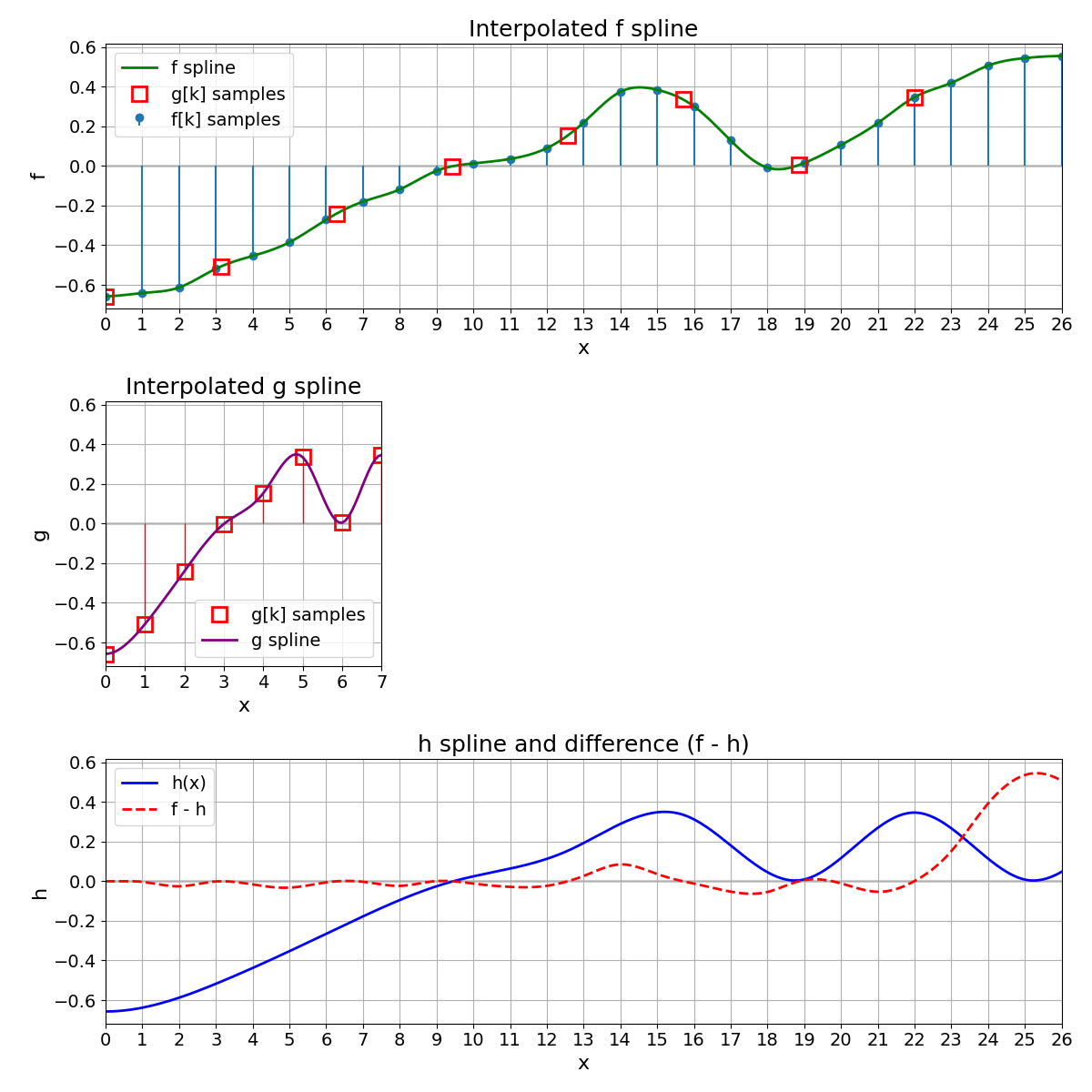
Expand g to Obtain h

To compare \(g\) on the same domain as \(f\), we expand \(g\) by defining a new function \(h\) as

\[h(x) = g\bigl(\tfrac{x}{T}\bigr),\]

where \(g\) is the continuously defined spline built from the discrete points \(g[k]\). Hence, \(h\) and \(f\) have the same support and can be directly compared (e.g., by computing an MSE).

fig2 = plt.figure(figsize=(12, 12))

gs2 = GridSpec(
    nrows=3,
    ncols=2,
    width_ratios=[g_support_length, f_support_length - g_support_length],
    height_ratios=[1, 1, 1]  # three equal rows
)

# TOP ROW: f + f spline + discrete g[k]
ax_top = fig2.add_subplot(gs2[0, :])  # spans both columns
ax_top.set_title("Interpolated f spline")

# Replot discrete f[k] as stems
ax_top.stem(f_support, f_samples, basefmt=" ", label="f[k] samples")

# Replot f spline
ax_top.plot(f_coords, f_data, color="green", linewidth=2, label="f spline")

# Overplot discrete g[k] in red squares at x = k*val_T
x_g = np.arange(g_support_length) * val_T
ax_top.plot(
    x_g, g_samples,
    "rs", mfc='none', markersize=12, markeredgewidth=2,
    label="g[k] samples"
)

# Horizontal line at 0
ax_top.axhline(0, color="black", linewidth=1, zorder=0)

ax_top.set_xlim(0, f_support_length - 1)
ax_top.set_xticks(np.arange(0, f_support_length, 1))
ax_top.set_xlabel("x")
ax_top.set_ylabel("f")
ax_top.legend()
ax_top.grid(True)

# MIDDLE ROW: discrete g + g spline
ax_mid_left = fig2.add_subplot(gs2[1, 0])  # left cell
ax_mid_right = fig2.add_subplot(gs2[1, 1]) # right cell
ax_mid_right.axis("off")                  # keep it blank

ax_mid_left.set_title("Interpolated g spline")

# Plot discrete g[k] with red stems, unfilled squares
ax_mid_left.vlines(
    x=g_support,
    ymin=0,
    ymax=g_samples,
    color='red',
    linestyle='-',
    linewidth=1
)
ax_mid_left.plot(
    g_support,
    g_samples,
    "rs", mfc='none', markersize=12, markeredgewidth=2,
    label="g[k] samples"
)

# Plot g spline
ax_mid_left.plot(
    g_coords, g_data,
    color="purple", linewidth=2,
    label="g spline"
)

ax_mid_left.axhline(0, color='black', linewidth=1, zorder=0)
ax_mid_left.set_xlim(0, g_support_length - 1)
ax_mid_left.set_xticks(np.arange(0, g_support_length, 1))
ax_mid_left.set_xlabel("x")
ax_mid_left.set_ylabel("g")
ax_mid_left.legend()
ax_mid_left.grid(True)

# Match y-limits with top row:
ax_mid_left.set_ylim(ax_top.get_ylim())

# BOTTOM ROW: expanded h(x) = g(x / λ)
ax_bottom = fig2.add_subplot(gs2[2, :])  # spans both columns
ax_bottom.set_title("h spline and difference (f - h)")

# We'll sample h over 0..(f_support_length-1)
h_coords = f_coords
# Evaluate h(x) = g(x/val_T)
h_data = g(coordinates=(h_coords / val_T,), grid=False)

# Also evaluate f at the same coords, so we can show the difference
f_data_for_diff = f(coordinates=(h_coords,), grid=False)
diff_data = f_data_for_diff - h_data

# Plot h in blue
ax_bottom.plot(h_coords, h_data, color="blue", linewidth=2, label="h(x)")

# Plot difference f - h in red, dashed
ax_bottom.plot(h_coords, diff_data, color="red", linestyle="--", linewidth=2, label="f - h")

ax_bottom.axhline(0, color='black', linewidth=1, zorder=0)

# The domain is the same as f
ax_bottom.set_xlim(0, f_support_length - 1)
ax_bottom.set_xticks(np.arange(0, f_support_length, 1))
ax_bottom.set_xlabel("x")
ax_bottom.set_ylabel("h")
ax_bottom.grid(True)
ax_bottom.legend()

# Match y axis with top row
ax_bottom.set_ylim(ax_top.get_ylim())

fig2.tight_layout()
plt.show()

MSE Between f and h

We compute the MSE between \(h(x)\) and \(f(x)\) as

\[\text{MSE} = \frac{1}{b - a} \int_{a}^{b} (f(x) - h(x))^2 \, \mathrm{d}x.\]

Riemann Approximation

To estimate this integral, we discretize the interval \([a,b]\) into \(K\) points. At each point \(x_k\), we evaluate \((f(x_k) - h(x_k))^2\) and multiply by the width \(\Delta x\). Summing across all points produces the approximation

\[\Delta x \sum_{k=1}^{K} (f(x_k) - h(x_k))^2 \;\approx\; \int_{a}^{b} (f(x) - h(x))^2 \, \mathrm{d}x.\]

The normalization by \((b-a)\) yields the MSE.

# 1) Define a midpoint sampling domain for [a, b]
N = 1000
padding_fraction = 0.2 # We avoid artifacts near the edges by excluding part of the domain from each side
a = (f_support_length - 1) * padding_fraction
b = (f_support_length - 1) * (1 - padding_fraction)
dx = (b - a) / N
mid_x = np.linspace(a + dx/2, b - dx/2, N)  # midpoints

# 2) Evaluate f(x) and h(x) at those midpoints
f_mid = f(coordinates=(mid_x,), grid=False)
h_mid = g(coordinates=(mid_x / val_T,), grid=False)

# 3) Compute the midpoint Riemann sum for ∫(f(x)-h(x))^2 dx
squared_diff = (f_mid - h_mid) ** 2
integral_value = np.sum(squared_diff) * dx

# 4) Divide by (b - a) to get the MSE
mse_midpoint = integral_value / (b - a)
print(f"MSE between f and h = {mse_midpoint:.6e}")

MSE between f and h = 1.152514e-03

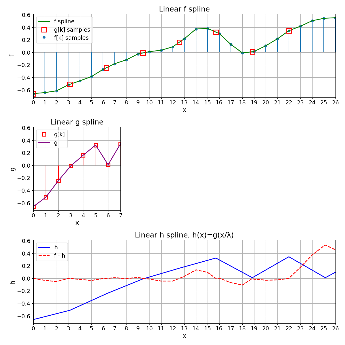
Variation with Linear Splines

We repeat exactly everything with linear splines. As the MSE increases, we conclude that splines of degree 3 provide a better representation of the original signal than splines of degree 1.

base = "bspline1"
mode = "mirror"

# 1) Rebuild linear-spline version of f, then g
f_lin = TensorSpline(data=f_samples, coordinates=f_support, bases=base, modes=mode)
g_lin_samps = f_lin(coordinates=(f_resampled_coords,), grid=False)
g_lin = TensorSpline(data=g_lin_samps, coordinates=g_support, bases=base, modes=mode)

# 2) Evaluate them at the same plotting coordinates
f_lin_f = f_lin(coordinates=(f_coords,), grid=False)               # f_lin over domain 0..(K-1)
g_lin_g = g_lin(coordinates=(g_coords,), grid=False)               # g_lin over domain 0..(g_support_length-1)
h_lin_h = g_lin(coordinates=(f_coords / val_T,), grid=False)  # h_lin(x)=g_lin(x/λ) over 0..(K-1)

# 3) Create the 3×2 figure layout
fig3 = plt.figure(figsize=(12, 12))
gs3 = GridSpec(
    nrows=3,
    ncols=2,
    width_ratios=[g_support_length, f_support_length - g_support_length],
    height_ratios=[1, 1, 1]
)

# TOP ROW: entire row (two columns combined) for f
ax_top = fig3.add_subplot(gs3[0, :])
ax_top.set_title("Linear f spline")

# Plot f[k] as stems
ax_top.stem(f_support, f_samples, basefmt=" ", label="f[k] samples")

# Plot f spline
ax_top.plot(f_coords, f_lin_f, color="green", linewidth=2, label="f spline")

# Overplot discrete g[k] as unfilled red squares at x = k * val_T
x_g = np.arange(g_support_length) * val_T
ax_top.plot(
    x_g, g_lin_samps,
    "rs",              # red squares
    mfc='none',        # unfilled
    markersize=12,
    markeredgewidth=2,
    label="g[k] samples"
)

ax_top.axhline(0, color='black', linewidth=1, zorder=0)
ax_top.set_xlim(0, f_support_length - 1)
ax_top.set_xticks(np.arange(0, f_support_length, 1))
ax_top.set_xlabel("x")
ax_top.set_ylabel("f")
ax_top.grid(True)
ax_top.legend()

# MIDDLE ROW: left subplot shows g domain, right subplot is blank
ax_mid_left = fig3.add_subplot(gs3[1, 0])
ax_mid_right = fig3.add_subplot(gs3[1, 1])
ax_mid_right.axis("off")  # keep right side blank

ax_mid_left.set_title("Linear g spline")

# Discrete g[k] with stems
ax_mid_left.vlines(
    x=g_support,
    ymin=0,
    ymax=g_lin_samps,
    color='red',
    linewidth=1
)
ax_mid_left.plot(
    g_support,
    g_lin_samps,
    "rs", mfc='none', markersize=8, markeredgewidth=2,
    label="g[k]"
)
# g spline
ax_mid_left.plot(
    g_coords,
    g_lin_g,
    color="purple", linewidth=2,
    label="g"
)
ax_mid_left.axhline(0, color='black', linewidth=1, zorder=0)
ax_mid_left.set_xlim(0, g_support_length - 1)
ax_mid_left.set_xticks(np.arange(0, g_support_length, 1))
ax_mid_left.set_xlabel("x")
ax_mid_left.set_ylabel("g")
ax_mid_left.grid(True)
ax_mid_left.legend()
# Match y-range with top
ax_mid_left.set_ylim(ax_top.get_ylim())

# BOTTOM ROW: entire row for h
ax_bottom = fig3.add_subplot(gs3[2, :])
ax_bottom.set_title("Linear h spline, h(x)=g(x/λ)")

ax_bottom.plot(f_coords, h_lin_h, color="blue", linewidth=2, label="h")

# Evaluate f_lin at the same coords, then difference
f_lin_for_diff = f_lin(coordinates=(f_coords,), grid=False)
diff_lin = f_lin_for_diff - h_lin_h

# Plot difference in red, dashed
ax_bottom.plot(f_coords, diff_lin, color="red", linestyle="--", linewidth=2, label="f - h")

ax_bottom.axhline(0, color='black', linewidth=1, zorder=0)
ax_bottom.set_xlim(0, f_support_length - 1)
ax_bottom.set_xticks(np.arange(0, f_support_length, 1))
ax_bottom.set_xlabel("x")
ax_bottom.set_ylabel("h")
ax_bottom.grid(True)
ax_bottom.legend()
ax_bottom.set_ylim(ax_top.get_ylim())

fig3.tight_layout()
plt.show()

# 4) Recompute MSE with linear splines using midpoint rule
N = 1000
padding_fraction = 0.2 # We avoid artifacts near the edges by excluding part of the domain from each side
a = (f_support_length - 1) * padding_fraction
b = (f_support_length - 1) * (1 - padding_fraction)
dx = (b - a) / N

# mid_x are the midpoints of each subinterval
mid_x = np.linspace(a + dx/2, b - dx/2, N)

# Evaluate f_lin and h_lin at midpoints
f_lin_mid = f_lin(coordinates=(mid_x,), grid=False)
h_lin_mid = g_lin(coordinates=(mid_x / val_T,), grid=False)

# Midpoint Riemann sum for ∫(f_lin - h_lin)²
squared_diff_lin = (f_lin_mid - h_lin_mid) ** 2
integral_value_lin = np.sum(squared_diff_lin) * dx

# Divide by (b - a) to get MSE
mse_lin_midpoint = integral_value_lin / (b - a)
print(f"MSE with linear splines = {mse_lin_midpoint:.6e}")

MSE with linear splines = 2.604823e-03