1D Fractional Brownian Motion

We use the smooth module to smooth a 1D fractional Brownian motion signal.

Imports

import math
import numpy as np
import matplotlib.pyplot as plt
from splineops.denoise.fBmper import fBmper
from splineops.denoise.smoothing_spline import smoothing_spline

1D Fractional Brownian Motion

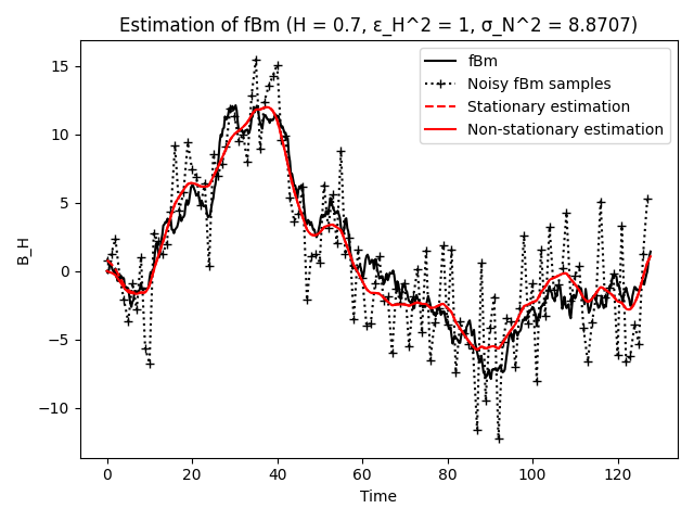
A realization of an fBm process of length N is generated and corrupted with noise. The sequence is then denoised and oversampled by a factor m using the optimal fractional-spline estimator.

# Define program constants
m = 4       # Upsampling factor
N = 256     # Number of samples

# Default values
default_H = 0.7
default_SNRmeas = 20.0
default_verify = '0'

# Enter Hurst parameter [0 < H < 1] (default: 0.7) >
H = 0.7

# Enter measurement SNR at the mid-point (t = {N/2}) [dB] (default: 20.0) >
SNRmeas = 20.0

# Create pseudo-fBm signal
epsH = 1
t0, y0 = fBmper(epsH, H, m, N)
Ch = epsH ** 2 / (math.gamma(2 * H + 1) * np.sin(np.pi * H))
POWmid = Ch * (N / 2) ** (2 * H)  # Theoretical fBm variance at the midpoint

# Measurement: downsample and add noise
t = t0[::m]
y = y0[::m]
sigma = np.sqrt(POWmid) / (10 ** (SNRmeas / 20))
noise = np.random.randn(N)
noise = sigma * noise / np.sqrt(np.mean(noise ** 2))
y_noisy = y + noise

# Find smoothing spline fit
lambda_ = (sigma / epsH) ** 2
gamma_ = H + 0.5
ts, ys = smoothing_spline(y_noisy, lambda_, m, gamma_)

# Add non-stationary correction term
cnn = np.concatenate(([1], np.zeros(N - 1)))  # Normalized white noise autocorrelation
tes, r = smoothing_spline(cnn, lambda_, m, gamma_)
r = r * ys[0] / r[0]
y_est = ys - r

# Calculate MSE and SNR
MSE0 = np.mean(noise ** 2)                       # Measurement MSE
MSE = np.mean((y_est[::m] - y0[::m]) ** 2)       # Denoised sequence MSE
MSEm = np.mean((y_est - y0) ** 2)                # Denoised and oversampled signal MSE

SNR0 = 10 * np.log10(POWmid / MSE0)
SNR = 10 * np.log10(POWmid / MSE)
SNRm = 10 * np.log10(POWmid / MSEm)

print(f'Number of measurements is {N}, oversampling factor is {m}.')
print(f'mSNR (SNR at the mid-point) of the measured sequence      is {SNR0:.2f} dB.')
print(f'mSNR improvement of the denoised sequence                 is {SNR - SNR0:.2f} dB.')
print(f'mSNR improvement of the denoised and oversampled sequence is {SNRm - SNR0:.2f} dB.')

# Plot the results
plt.figure()
plt.plot(t0[:len(t0)//2], y0[:len(y0)//2], 'k', label='fBm')
plt.plot(t[:len(t)//2], y_noisy[:len(y_noisy)//2], 'k+:', label='Noisy fBm samples')
plt.plot(ts[:len(ts)//2], ys[:len(ys)//2], 'r--', label='Stationary estimation')
plt.plot(tes[:len(tes)//2], y_est[:len(y_est)//2], 'r', label='Non-stationary estimation')
plt.legend()
plt.title(f'Estimation of fBm (H = {H}, ε_H^2 = {epsH}, σ_N^2 = {sigma ** 2:.4f})')
plt.xlabel('Time')
plt.ylabel('B_H')
plt.tight_layout()
plt.show()

Number of measurements is 256, oversampling factor is 4.
mSNR (SNR at the mid-point) of the measured sequence      is 20.00 dB.
mSNR improvement of the denoised sequence                 is 7.57 dB.
mSNR improvement of the denoised and oversampled sequence is 7.71 dB.