Differentiate Module

In this example, we demonstrate how to use the differentiate module to compute different differential operations on an image.

Imports

import numpy as np
import matplotlib.pyplot as plt
from mpl_toolkits.axes_grid1 import make_axes_locatable
import requests
from io import BytesIO
from PIL import Image

# Import the Differentials class from your module (adjust import path as needed)
from splineops.differentiate.differentials import differentials

Data Preparation

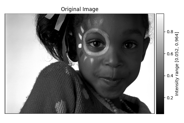
We retrieve an example color image, convert it to grayscale, and normalize its intensities to the [0,1] range.

url = 'https://r0k.us/graphics/kodak/kodak/kodim15.png'
response = requests.get(url)
img = Image.open(BytesIO(response.content))
image = np.array(img, dtype=np.float64)

# Convert to [0,1]
image_normalized = image / 255.0

# Convert to grayscale via simple weighting
image_gray = (
    image_normalized[:, :, 0] * 0.2989 +
    image_normalized[:, :, 1] * 0.5870 +
    image_normalized[:, :, 2] * 0.1140
)

Helper Visualization Functions

def show_result_with_colorbar(title, result, units="Value", percentile_range=(5, 95)):
    """
    Displays a 2D result with a colorbar scaled using the given percentile range.

    Parameters
    ----------
    title : str
        Title for the plot.
    result : ndarray
        2D array representing the image or field to display.
    units : str
        Label for the colorbar (e.g., 'Intensity', 'Radians', etc.).
    percentile_range : tuple or None
        Percentiles to use for scaling the colormap. If None, use the min and max of the data.
    """
    h, w = result.shape
    aspect_ratio = h / float(w)
    fig_width = 6.0
    fig_height = fig_width * aspect_ratio
    fig, ax = plt.subplots(figsize=(fig_width, fig_height))

    # Determine vmin and vmax based on percentiles if provided
    if percentile_range is not None:
        pmin, pmax = np.percentile(result, percentile_range)
        im = ax.imshow(result, cmap='gray', aspect='equal', vmin=pmin, vmax=pmax)
        cbar_label = f"{units} range [{pmin:.3f}, {pmax:.3f}]"
    else:
        vmin, vmax = result.min(), result.max()
        im = ax.imshow(result, cmap='gray', aspect='equal', vmin=vmin, vmax=vmax)
        cbar_label = f"{units} range [{vmin:.3f}, {vmax:.3f}]"

    ax.set_title(title)
    ax.axis('off')

    # Create a colorbar with matching height using make_axes_locatable
    divider = make_axes_locatable(ax)
    cax = divider.append_axes("right", size="5%", pad=0.05)
    cbar = plt.colorbar(im, cax=cax)
    cbar.set_label(cbar_label)

    plt.tight_layout()
    plt.show()


def show_angle_result(title, angle_data, vmin, vmax, units="Radians"):
    """
    Displays angle data in a cyclical color map (hsv), with vmin and vmax specifying
    the circular range.

    Parameters
    ----------
    title : str
        Title for the plot.
    angle_data : ndarray
        2D array of angles (in radians).
    vmin : float
        Minimum of angle range (e.g., 0).
    vmax : float
        Maximum of angle range (e.g., 2*pi).
    units : str
        Label for the colorbar (e.g., 'Direction (radians)', etc.).
    """
    h, w = angle_data.shape
    aspect_ratio = h / float(w)
    fig_width = 6.0
    fig_height = fig_width * aspect_ratio
    fig, ax = plt.subplots(figsize=(fig_width, fig_height))

    # Plot with an HSV cyclical colormap
    im = ax.imshow(angle_data, cmap='hsv', aspect='equal', vmin=vmin, vmax=vmax)
    ax.set_title(title)
    ax.axis('off')

    # Add colorbar
    divider = make_axes_locatable(ax)
    cax = divider.append_axes("right", size="5%", pad=0.05)
    cbar = plt.colorbar(im, cax=cax, ticks=[vmin, (vmin+vmax)/2, vmax])
    cbar.set_label(f"{units} range [{vmin:.2f}, {vmax:.2f}]")

    plt.tight_layout()
    plt.show()

Show the original grayscale image with a colorbar

show_result_with_colorbar("Original Image", image_gray, units="Intensity")

Gradient Magnitude

diff = differentials(image_gray.copy())
diff.run(differentials.GRADIENT_MAGNITUDE)
grad_magnitude_result = diff.image

show_result_with_colorbar("Gradient Magnitude", grad_magnitude_result, units="Value")

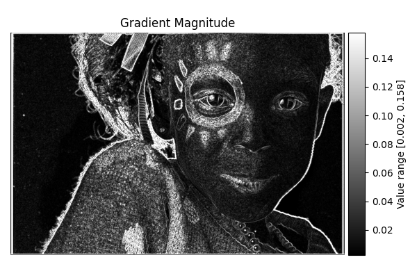
Completed in 1.16 seconds

Gradient Direction

diff = differentials(image_gray.copy())
diff.run(differentials.GRADIENT_DIRECTION)
grad_direction_result = diff.image

# Shift from [-π, π] to [0, 2π]
grad_direction_result_0_2pi = (grad_direction_result + 2.0*np.pi) % (2.0*np.pi)

# Visualize with HSV colormap, removing percentile clipping
show_angle_result(
    "Gradient Direction",
    grad_direction_result_0_2pi,
    vmin=0.0, vmax=2.0*np.pi,
    units="Direction (radians)"
)

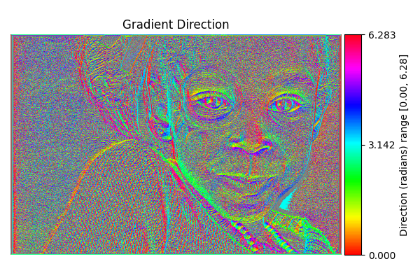
Completed in 1.14 seconds

Laplacian

diff = differentials(image_gray.copy())
diff.run(differentials.LAPLACIAN)
laplacian_result = diff.image

show_result_with_colorbar("Laplacian", laplacian_result, units="Value")

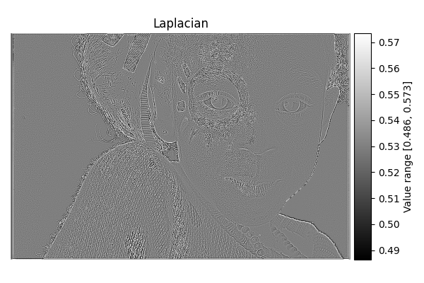
Completed in 1.35 seconds

Largest Hessian

diff = differentials(image_gray.copy())
diff.run(differentials.LARGEST_HESSIAN)
largest_hessian_result = diff.image

show_result_with_colorbar("Largest Hessian Eigenvalue", largest_hessian_result, units="Value")

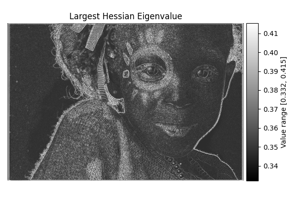
Completed in 2.52 seconds

Smallest Hessian

diff = differentials(image_gray.copy())
diff.run(differentials.SMALLEST_HESSIAN)
smallest_hessian_result = diff.image

show_result_with_colorbar("Smallest Hessian Eigenvalue", smallest_hessian_result, units="Value")

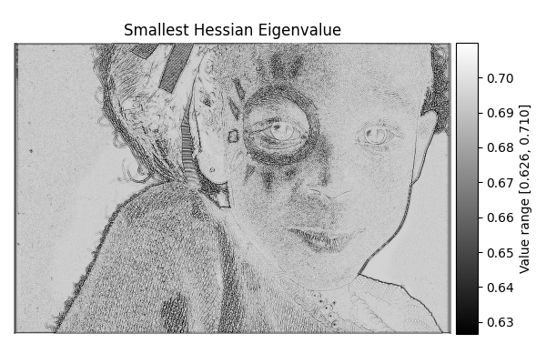
Completed in 2.45 seconds

Hessian Orientation

diff = differentials(image_gray.copy())
diff.run(differentials.HESSIAN_ORIENTATION)
hessian_orientation_result = diff.image

show_angle_result(
    "Hessian Orientation",
    hessian_orientation_result,
    vmin=-np.pi/2.0, vmax=np.pi/2.0,
    units="Orientation (radians)"
)

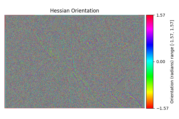
Completed in 2.50 seconds