Resize Module

Shrink and re-expand a 2-D RGB image with splineops, then discuss aliasing.

Imports

import numpy as np
import matplotlib.pyplot as plt
import requests
from io import BytesIO
from PIL import Image

from scipy.ndimage import zoom as ndi_zoom          # only for the *first* quick shrink
from splineops.utils import (
    adjust_size_for_zoom,   # makes dimensions compatible with the zoom factor
    resize_multichannel,    # channel-wise wrapper around splineops.resize
)

plt.rcParams.update({
    "font.size": 14,
    "axes.titlesize": 18,
    "axes.labelsize": 16,
})

Load and Normalize an Image

url = "https://r0k.us/graphics/kodak/kodak/kodim19.png"
img = Image.open(BytesIO(requests.get(url).content))
data = np.asarray(img, dtype=np.float64) / 255.0      # H × W × 3, range [0, 1]

# 1) Quick down-size so the notebook images aren't huge
initial_shrink = 0.8
data_small = ndi_zoom(data, (initial_shrink, initial_shrink, 1), order=1)

# 2) Choose the demo shrink factor and make dimensions "zoom-friendly"
shrink_factor = 0.3
adjusted = adjust_size_for_zoom(data_small, shrink_factor)      # still float64 [0, 1]
adjusted_uint8 = (adjusted * 255).astype(np.uint8)

# 3) Shrink with splineops
shrunken = resize_multichannel(
    adjusted,               # float64 [0, 1]
    shrink_factor,
    method="cubic",          # plain cubic interpolation
    modes="mirror",
)                           # returns uint8

# Put the shrunken image on a white canvas the size of *adjusted*
H_adj, W_adj, _ = adjusted_uint8.shape
canvas = np.full_like(adjusted_uint8, 255)
canvas[: shrunken.shape[0], : shrunken.shape[1]] = shrunken

# 4) Re-expand to the original adjusted size
expanded = resize_multichannel(
    shrunken.astype(np.float64) / 255.0,   # back to float64 [0, 1]
    1.0 / shrink_factor,
    method="cubic",
    modes="mirror",
)

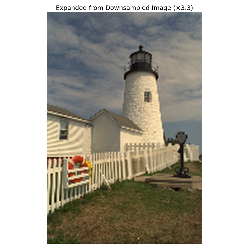
Expanded from Downsampled

We first show the final expanded image at large scale. This helps Sphinx generate a visually useful thumbnail and lets users preview the aliasing artefacts up front.

plt.figure(figsize=(10, 10))  # Tune size for thumbnail quality
plt.imshow(expanded)
plt.title(f"Expanded from Downsampled Image (×{1/shrink_factor:.1f})", fontsize=18)
plt.axis("off")
plt.tight_layout()
plt.show()

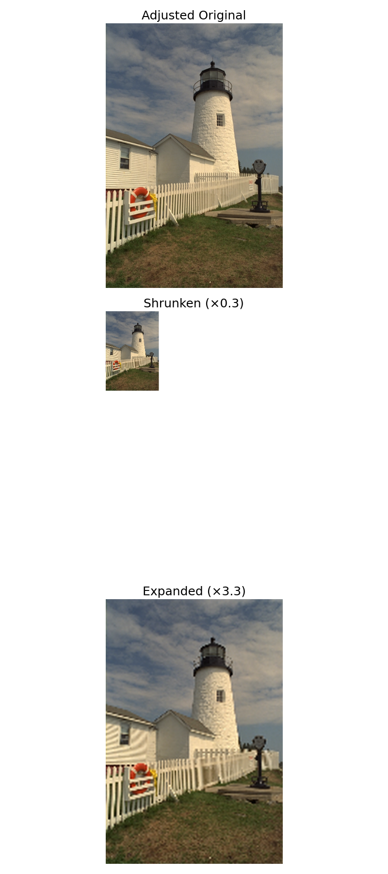
Resize Stages

We go through the stages of shrinking the image and then expanding it.

fig, axes = plt.subplots(3, 1, figsize=(8, 18))
axes[0].imshow(adjusted_uint8);
axes[0].set_title("Adjusted Original"); axes[0].axis("off")
axes[1].imshow(canvas);
axes[1].set_title(f"Shrunken (×{shrink_factor})"); axes[1].axis("off")
axes[2].imshow(expanded);
axes[2].set_title(f"Expanded (×{1/shrink_factor:.1f})"); axes[2].axis("off")
plt.tight_layout(); plt.show()

Aliasing discussion

Note the wave-like artefacts in the expanded image: classic aliasing. When we shrink below the Nyquist limit, high-frequency detail folds back into lower frequencies. Upsampling cannot recover the lost detail, so those aliased components become Moiré-style patterns. A proper workflow would low-pass filter before down-sampling, but here we purposely show the artefacts to illustrate the point.