Compare Different Methods

A summary of the cost/benefit tradeoff of the three interpolation methods is provided in this example.

Imports

import numpy as np
import matplotlib.pyplot as plt
import requests
from io import BytesIO
from PIL import Image

from splineops.utils import (
    resize_and_compute_metrics,      # resampling + metrics
    show_roi_zoom,
)

Load and Normalize an Image

Here, we load an example image from an online repository. We convert it to grayscale in [0, 1].

url = 'https://r0k.us/graphics/kodak/kodak/kodim14.png'
response = requests.get(url)
img = Image.open(BytesIO(response.content))
data = np.array(img, dtype=np.float64)

# Convert to [0..1]
input_image_normalized = data / 255.0

# Convert to grayscale via simple weighting
input_image_normalized = (
    input_image_normalized[:, :, 0] * 0.2989 +  # Red channel
    input_image_normalized[:, :, 1] * 0.5870 +  # Green channel
    input_image_normalized[:, :, 2] * 0.1140    # Blue channel
)

zoom_factors_2d = (0.25, 0.25)
border_fraction = 0.3

# --- ROI: match the LS/Oblique examples ---
ROI_SIZE_PX = 64
FACE_ROW, FACE_COL = 400, 600  # ROI center in ORIGINAL coordinates

h_img, w_img = input_image_normalized.shape
row_top  = int(np.clip(FACE_ROW - ROI_SIZE_PX // 2, 0, h_img - ROI_SIZE_PX))
col_left = int(np.clip(FACE_COL - ROI_SIZE_PX // 2, 0, w_img - ROI_SIZE_PX))
roi_rect = (row_top, col_left, ROI_SIZE_PX, ROI_SIZE_PX)  # (r, c, h, w)

# Reusable kwargs for consistent ROI zooms below
roi_kwargs = dict(
    roi_height_frac=ROI_SIZE_PX / h_img,
    grayscale=True,
    roi_xy=(row_top, col_left),
)

Standard Interpolation

We use our standard interpolation method.

(
    resized_2d_interp,
    recovered_2d_interp,
    snr_2d_interp,
    mse_2d_interp,
    time_2d_interp
) = resize_and_compute_metrics(
    input_image_normalized,
    method="cubic",
    zoom_factors=zoom_factors_2d,
    border_fraction=border_fraction,
    roi=roi_rect,  # <-- compute metrics on the shared ROI
)

Least-Squares Projection

We use the least-squares projection method.

(
    resized_2d_ls,
    recovered_2d_ls,
    snr_2d_ls,
    mse_2d_ls,
    time_2d_ls
) = resize_and_compute_metrics(
    input_image_normalized,
    method="cubic-best_antialiasing",
    zoom_factors=zoom_factors_2d,
    border_fraction=border_fraction,
    roi=roi_rect,  # <-- compute metrics on the shared ROI
)

Oblique Projection

We use the oblique-projection method.

(
    resized_2d_ob,
    recovered_2d_ob,
    snr_2d_ob,
    mse_2d_ob,
    time_2d_ob
) = resize_and_compute_metrics(
    input_image_normalized,
    method="cubic-fast_antialiasing",
    zoom_factors=zoom_factors_2d,
    border_fraction=border_fraction,
    roi=roi_rect,  # <-- compute metrics on the shared ROI
)

Comparison

We compare the performance of the different methods being analyzed.

Comparison Table

We print the SNR, MSE, and timing data for each method.

methods = [
    ("Standard Interpolation", snr_2d_interp, mse_2d_interp, time_2d_interp),
    ("Least-Squares Projection", snr_2d_ls, mse_2d_ls, time_2d_ls),
    ("Oblique Projection", snr_2d_ob, mse_2d_ob, time_2d_ob),
]

# Print the table header using the same widths as we'll use for data
header_line = f"{'Method':<25} {'SNR (dB)':>10} {'MSE':>16} {'Time (s)':>12}"
print(header_line)
print("-" * len(header_line))  # or manually set a dash length, e.g. 67

# Now print each row with the matching format
for method_name, snr_val, mse_val, time_val in methods:
    row_line = f"{method_name:<25} {snr_val:>10.2f} {mse_val:>16.2e} {time_val:>12.4f}"
    print(row_line)

Method                      SNR (dB)              MSE     Time (s)
------------------------------------------------------------------
Standard Interpolation         12.15         2.20e-02       0.0187
Least-Squares Projection       14.28         1.35e-02       1.4392
Oblique Projection             14.24         1.36e-02       1.1208

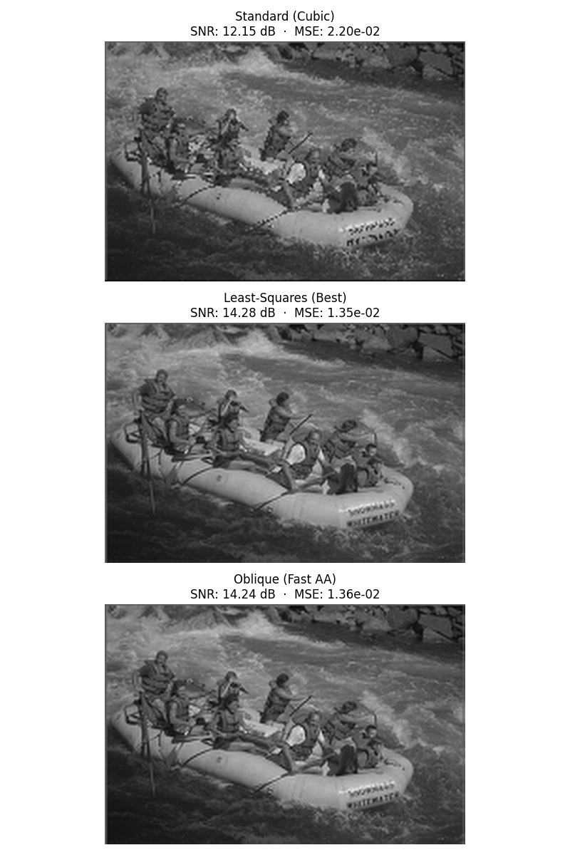
All Methods

recovered_stack = [
    ("Standard (Cubic)",       recovered_2d_interp, snr_2d_interp, mse_2d_interp),
    ("Least-Squares (Best)",   recovered_2d_ls,     snr_2d_ls,     mse_2d_ls),
    ("Oblique (Fast AA)",      recovered_2d_ob,     snr_2d_ob,     mse_2d_ob),
]

fig, axes = plt.subplots(3, 1, figsize=(8, 12))

for ax, (label, img, snr_val, mse_val) in zip(axes, recovered_stack):
    ax.imshow(img, cmap="gray", aspect="equal")
    ax.set_title(f"{label}\nSNR: {snr_val:.2f} dB  ·  MSE: {mse_val:.2e}")
    ax.axis("off")

plt.tight_layout()
plt.show()

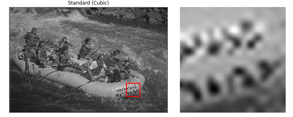
Standard Interpolation

_ = show_roi_zoom(
    recovered_2d_interp,     # image to inspect
    ax_titles=("Standard (Cubic)", None),  # customise left title; right auto
    **roi_kwargs
)

Least-Squares Projection

_ = show_roi_zoom(
    recovered_2d_ls,     # image to inspect
    ax_titles=("Least-Squares (Best)", None),  # customise left title; right auto
    **roi_kwargs
)

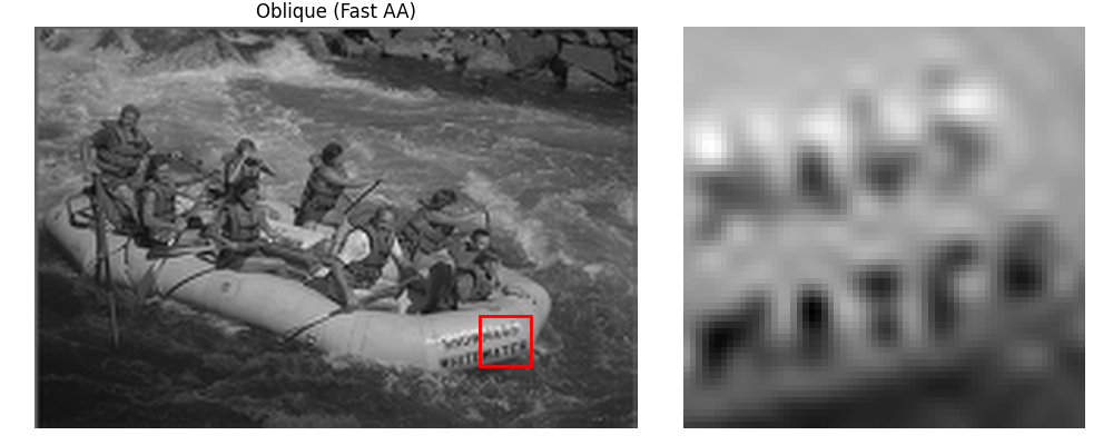
Oblique Projection

_ = show_roi_zoom(
    recovered_2d_ob,     # image to inspect
    ax_titles=("Oblique (Fast AA)", None),  # customise left title; right auto
    **roi_kwargs
)